4.8.4 Three-Dimensional Temperature Distribution

The following example is mainly intended for a comparative study of performance and memory management of AMIGOS. Although such comparisons are not really expressive they give an idea about the performance of the system. As a comparative tool an existing highly optimized `hand coded' finite element solver (STAP - SMART THERMAL ANALYSIS PROGRAM [Bau94][Sta97][Sab98]) has been chosen since internal knowledge about STAP is available and performance differences can be estimated better.

STAP is a simulation tool which allows transient and static thermal analysis of interconnects under electrical stress. A preconditioned conjugate gradient method is implemented to solve the large linear system in order to obtain the distributions of potential and temperature. To achieve an efficient utilization of computer memory, a compressed matrix format for the sparsely occupied stiffness matrix is used.

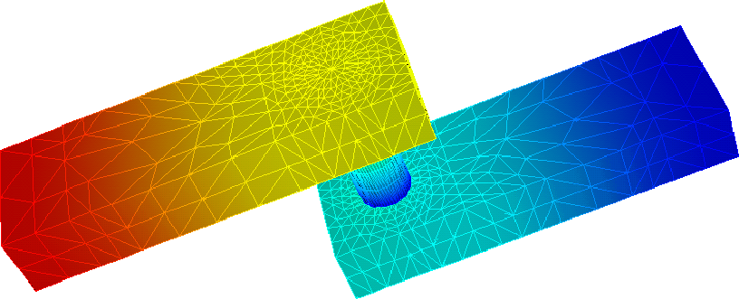
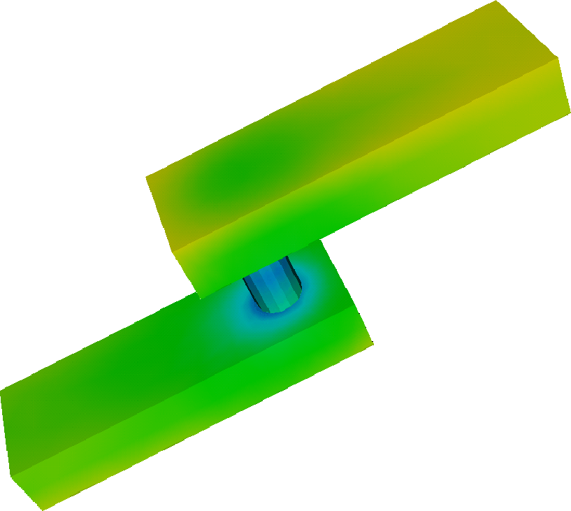
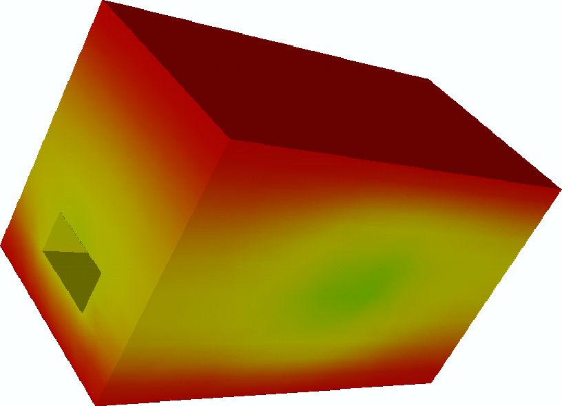
A two layer interconnect structure has been chosen as benchmark example where temperature and potential distributions are calculated.

The model for the numerical calculation of joule self heating effects is based on two partial differential equations. First, the heat-conduction equation

$$\rho {\frac{\partial T}{\partial t}} \left(\vphantom{\gamma_T \cdot grad (T)}\right. \gamma_{T}^{} \left.\vphantom{\gamma_T \cdot grad (T)}\right)$$ (4.28)

has to be solved to calculate the temperature distribution T in conductor and insulator domains, where c_p is the specific heat and $\rho$ is the mass density of the material. $\gamma_{T}^{}$ represents the material specific thermal conductivity, t is the time, and the term on the right side p is the electrical power loss density.

For stationary problems the heat-conduction equation can be simplified to

$$\left(\vphantom{\gamma_T \cdot grad (T)}\right. \gamma_{T}^{} \left.\vphantom{\gamma_T \cdot grad (T)}\right)$$ (4.29)

The power loss density p is derived from the electric potential $\varphi$

$$\gamma_{E}^{} \left(\vphantom{ grad (\varphi) }\right. \varphi \left.\vphantom{ grad (\varphi) }\right)^{2}_{}$$ (4.30)

that is calculated by solving the Euler Equation

$$\left(\vphantom{ \gamma \cdot grad (\varphi)}\right. \gamma \varphi \left.\vphantom{ \gamma \cdot grad (\varphi)}\right)$$ (4.31)

The electrical conductivity which in this case is a function of the temperature will be modeled by

$$\gamma \gamma_{0}^{} {\frac{1}{1+\alpha \left(T-T_0\right)}}$$ (4.32)

In this model the dependence of $\gamma$ on the temperature T is determined by the coefficient $\alpha$. $\gamma_{0}^{}$ is the conductivity at the reference temperature T₀ of 300K.

The developed analytical model of AMI looks like:

MODEL PowerLoss_Temperature = [U,T];   # the solution vector
{
####### The Three-Dimensional Finite Element Discretization #########

    N(xsi,eta,zta) = [ 1 - xsi - eta - zta , xsi , eta , zta ];
    dN             = [[ -1 , 1 , 0 , 0 ]
                      [ -1 , 0 , 1 , 0 ]
                      [ -1 , 0 , 0 , 1 ]];
    x = [[X,Y,Z]];         
    dxdxsi = dN * x;       
    detJ   = |dxdxsi|;
    dxsidx = Inv(dxdxsi);
    dNdX = dxsidx*dN;
    i = 1..4;
######################### The Parameters ############################

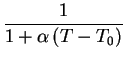
    Param alpha    = 0.0043;            
    Param gam_el   = 4.17;              
    Param gam_300  = 222.0E-6;          
    gam(T) = gam300/(1+alpha*(T-300)); 
    gam_th = 1/4 * Sum{i}(gam(T[i]));

################### The Differential Equations ######################

    K(gamma) = dNdX^T * gamma * dNdX;     # laplace operator in 
                                          # dependence of the value of 
                                          # gamma
    p1[i] = 0;                            # define a zero-vector of 
                                          # size 1x4
    E  = dNdX*U;                          # the electrical field
    p2 = gam_el*N(1/4,1/4,1/4)^T*(E^T*E); # the power loss density
    K = [[ K(gam_el) ,         O]         # disctretized laplace
         [     O     , K(gam_th)]];       # operators for both
                                          # quantities
############ The Residuum Vector and its Jacobian Matrix ############

    residuum = detJ*(K*[[U][T]]-[[p1][p2]]);
    jacobian = D([[U][T]],residuum^T)^T;
}

Figure 4.26: Performance comparison concerning calculation time and memory consumption

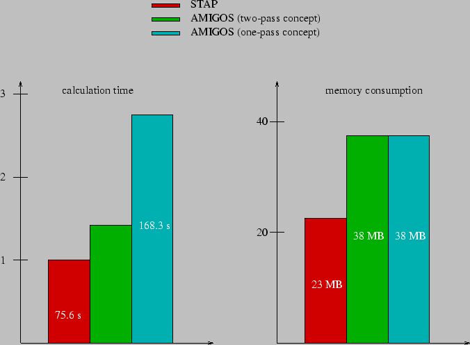
The comparisons (Fig. 4.26 and Fig. 4.27) were made calculating 14863 nodes building 73728 tetrahedrons (the calculated results are shown in Fig. 4.28, Fig. 4.29 and Fig. 4.30). The example was set up so that both systems needed three iterations to converge. Due to the different approaches to solve the differential equation systems within the two simulators it turned out that AMIGOS gains on performance with increasing non linearity. This is an effect due to the implicit dependence definition of the quantities using the analytical model interface. This approach has the disadvantage that the memory consumption of AMIGOS is much higher. Furthermore, STAP exploits the symmetry of the resulting sparse matrix for compression methods which is not used by AMIGOS for the sake of flexibility. Fig. 4.26 depicts the performance and memory comparisons related to the STAP solver.

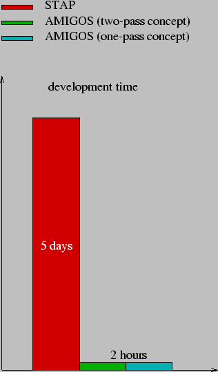
As expected AMIGOS cannot compete with optimized algorithms specialized to definite problems, although the demonstrated comparisons are satisfying and a lot of effort has been invested for high performance. However, a factor that can not be beaten by any other `hand-coded' algorithm shows Fig. 4.27. The development time of a new model has been compared where both scientists (developer of AMIGOS and developer of STAP) are already highly familiar with their algorithms thus the break-in period is negligible. The goal was to implement a transient electric simulation which was in scope of feasibility for the STAP system otherwise the differences in the result would be much higher.

Figure 4.27: Performance comparison concerning development time

Figure 4.28: Calculated potential distribution showing the mesh of discretization

Figure 4.29: Calculated temperature distribution within the two layered interconnected structure

Figure 4.30: Calculated temperature distribution within the surrounding insulator