2.3 Delaunay Elements and Meshes

Another very powerful element property for simplex elements is the Delaunay property [31].

Figure 2.11: Delaunay property

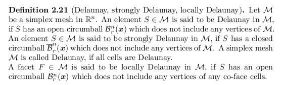
In the upper picture, a triangle (colored in blue) which is Delaunay in the mesh is shown. The lower picture visualizes a triangle (colored in blue) which is not Delaunay due to the red vertex which is inside the triangle's circumball and therefore breaks the Delaunay property of the triangle.

The Delaunay property is visualized in Figure 2.11. While the Delaunay property is a global property (all mesh vertices have to be checked), locally Delaunay only requires the evaluation of boundary vertices of neighbor simplices. Locally Delaunay is a weaker property for simplex elements than Delaunay, but if all facets of a mesh are locally Delaunay, the cells are in fact Delaunay.

Lemma 5 (Delaunay Lemma)   Let ${\mathcal{M}}$ be a simplex mesh in ${\mathbb{R}}^n$ with ${{\operatorname{DIM}}_{\operatorname{cell}}}({\mathcal{M}}) = n$, the following statements are equivalent:

• ${\mathcal{M}}$ is Delaunay.
• Every facet of ${\mathcal{M}}$ is Delaunay in ${\mathcal{M}}$.
• Every facet of ${\mathcal{M}}$ is locally Delaunay in ${\mathcal{M}}$.

A proof for this Lemma can be found in [127]. The Delaunay Lemma guarantees that the locally Delaunay property of facets, which is easier and more efficient to evaluate, results in the Delaunay property for cells. For each finite point set $S \subseteq {\mathbb{R}}^n$, there always exists a triangulation of $S$, which is Delaunay.

Delaunay is a very strong property for simplex meshes. For a simplex mesh ${\mathcal{M}}$ which is Delaunay, the dual is equal to the Voronoi diagram of ${\mathcal{M}}$. Some discretization-based simulation methods, like the FVM, utilize the Voronoi diagram during the discretization process [127]. For a given point set $S = \{\bm{s}_1, \dots, \bm{s}_k\} \subseteq {\mathbb{R}}^2$, a Delaunay triangulation ${\mathcal{M}}$ of $S$ maximizes the minimum angle and minimizes the largest circumball [127]. Unfortunately, this is not true for Delaunay triangulations in ${\mathbb{R}}^3$. To improve the quality of these meshes, post-processing, like mesh adaptation, is required. Additionally, a Delaunay triangulation minimizes the largest min-containment ball for arbitrary dimensions $n$ [136].

For a mesh ${\mathcal{M}}$ which is generated based on a PLC ${{\mathcal{P}}}$, a weaker Delaunay definition is of advantage.

Figure 2.12: Constrained Delaunay property

The blue triangle certainly is not Delaunay, because there are four vertices (indicated by red circles) which lie within the triangle's circumball. However, the triangle is constrained Delaunay, because the PLC boundary blocks the visibility of these vertices to the triangle.

A simplex which is constrained Delaunay, therefore is Delaunay except for vertices where the visibility is blocked by the PLC, e.g., on internal interfaces. An example visualizing the constrained Delaunay property is given in Figure 2.12. A Lemma similar to the Delaunay Lemma can be formulated for the constrained Delaunay property.

Lemma 6 (Constrained Delaunay Lemma)   Let ${\mathcal{M}}$ be a simplex mesh in ${\mathbb{R}}^n$ with ${{\operatorname{DIM}}_{\operatorname{cell}}}({\mathcal{M}}) = n$. Then, the following statements are equivalent.

• ${\mathcal{M}}$ is constrained Delaunay.
• Every facet of ${\mathcal{M}}$ which is not included in any facet of $P$ is constrained Delaunay in ${\mathcal{M}}$.
• Every facet of ${\mathcal{M}}$ which is not included in any facet of $P$ is locally Delaunay in ${\mathcal{M}}$.

As for the Delaunay Lemma, a proof for this Lemma is given in [127]. A multi-region mesh ${({\mathcal{M}}, {\xi})}$ is Delaunay, if all facets included in any PLC facet are locally Delaunay. For some PLCs it can be shown that there exists a triangulation which is constrained Delaunay.

For PLCs which are edge-protected, there is a guarantee for the existence of a mesh which is constrained Delaunay:

Lemma 7 (Constrained Delaunay mesh of edge-protected PLC)   Let ${({\mathcal{P}}, {\widetilde{\xi}})}$ be an edge-protected multi-region PLC. There is a triangulation ${({\mathcal{M}}, {\xi})}$ of the vertices of ${({\mathcal{P}}, {\widetilde{\xi}})}$ which is constrained Delaunay and geometry-conforms to ${({\mathcal{P}}, {\widetilde{\xi}})}$.

A proof for this Lemma can be found in [127]. For 2D PLCs in the plane there is an even stronger statement: Every multi-region PLC ${({\mathcal{P}}, {\widetilde{\xi}})}$ has a multi-region triangulation ${({\mathcal{M}}, {\xi})}$ of the vertices of ${({\mathcal{P}}, {\widetilde{\xi}})}$ which respects and geometry-conforms to ${({\mathcal{P}}, {\widetilde{\xi}})}$. However, in the 3D case, the edge-protected property is mandatory. To obtain a mesh which is Delaunay or constrained Delaunay, additional vertices have to be inserted. For every multi-region PLC, there exists a mesh which is Delaunay or constrained Delaunay [127].