6.3 Rotational Symmetries

The second main type of symmetries is the rotational symmetry.

A general rotation in ${\mathbb{R}}^2$ $\operatorname{rot}_{\bm{c}, \alpha}$ is given by a rotation center $\bm{c} \in {\mathbb{R}}^2$ and a rotation angle $\alpha \neq 0 \mod 360\degree$. In ${\mathbb{R}}^3$, an additional axis $\bm{v} \in {\mathbb{R}}^3$ is required to specify a rotation. Similar to reflections, a rotation has also fixed points being the rotation center $\bm{c}$ for rotations in ${\mathbb{R}}^2$ and every point on the rotation axis for rotations in ${\mathbb{R}}^3$. The general rotation in ${\mathbb{R}}^3$ can also be written in the following way [104]:

$$\operatorname{rot}_{\bm{c}, \bm{v}, \alpha} = R \begin{pmatrix}\c... ...ha) & \cos(\alpha) & 0\\ 0 & 0 & 1 \end{pmatrix} R^{-1}(\bm{x}-\bm{c}) + \bm{c}$$ (6.2)

with

$$R = {\mathbb{I}}+ G \sin(\theta) + G^2 (1-\cos(\theta))$$ (6.3)

$$\bm{t} = \bm{v} \times (0,0,1)^T$$ (6.4)

$$\theta = \cos^{-1}\left(\bm{v} \cdot (0,0,1)^T\right)$$ (6.5)

$$G = \begin{pmatrix} 0 & -t_z & t_y \\ t_z & 0 & -t_x \\ -t_y & t_x & 0 \end{pmatrix}$$ (6.6)

In this formulation of $\operatorname{rot}_{\bm{c}, \bm{v}, \alpha}$, $R$ specifies a coordinate system change, where the rotation is performed around the $z$-axis. A set is said to have a rotational symmetry of order $n$, if $n = 360\degree/\alpha$. Every set with a rotational symmetry of order $n$ has also a rotational symmetry of order $k$, if $k$ is a factor of $n$. Usually, a set with a rotational symmetry is specified using its largest symmetry order.

In contrast to reflective symmetries, there are infinitely many possible constructing subsets of a set having a rotational symmetry. Let $A$ be a set with a rotational symmetry of order $n$. Then any slice subset $S \subseteq A$ with an angle of $360\degree/n$ can be used to reconstruct $A$. A slice is defined as follows:

Figure 6.6: A slice of a set with a rotational symmetry

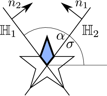
The slice starting angle is depicted as $\sigma$. The slice with a spanning angle of $\alpha$ is embedded between two hyperplanes with the normal vectors $\bm{n}_1$ and $\bm{n}_2$.

In other words, a slice is defined as all points which are on the positive side of two hyperplanes specified by the normal vectors $\bm{n}_1$ and $\bm{n}_2$. $\alpha$ is the spanning angle of the slice, i.e., the angle between the two hyperplanes, and $\sigma$ is the starting angle. A slice of an object in ${\mathbb{R}}^2$ is visualized in Figure 6.6.

Let $A \subseteq {\mathbb{R}}^2$ be a set with a rotational symmetry of order $n$ and center $\bm{c}$. $A$ can be reconstructed using a slice with any starting angle $\sigma$ in the following way:

$$A = \bigcup_{k=0}^{n-1} \operatorname{rot}_{\bm{c}, k\frac{360\degree}{n}} \left( {\mathcal{S}}_{\bm{c},\sigma,\alpha}(A) \right)$$ (6.7)

The same also works for $B \subseteq {\mathbb{R}}^3$ with a rotational symmetry of order $n$, center $\bm{c}$, and rotational axis $\bm{v}$:

$$B = \bigcup_{k=0}^{n-1} \operatorname{rot}_{\bm{c}, \bm{v}, k\frac{360\degree}{n}} \left( {\mathcal{S}}_{\bm{c},\bm{v},\sigma,\alpha}(B) \right)$$ (6.8)

Theoretically, the choice of the starting angle $\sigma$ is arbitrary. However, certain starting angles potentially have a bad impact on the element quality, like the smallest angle, of the resulting templated mesh. Therefore, the geometry has to be analyzed to determine good choices for $\sigma$. An algorithm which tackles this issue for linear geometries is presented in Section 6.3.1.

Figure 6.7: Boundary patch partition of a set with rotational symmetry

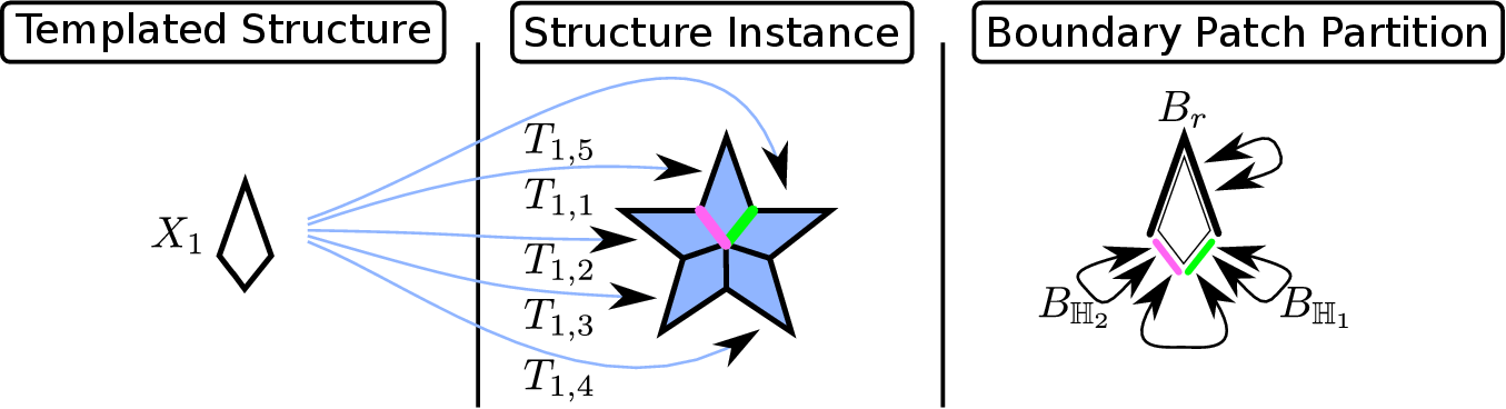
The boundary partition consists of three elements, being $B_{\mathbb{H}_1}$, $B_{\mathbb{H}_2}$, and $B_r$ where $B_{\mathbb{H}_1}$ and $B_{\mathbb{H}_2}$ are the only two different elements which are related to each other by the boundary patch relation.

Using the relation above, a geometry ${\mathcal{G}}$ with a rotational symmetry of order $n$, rotation center $\bm{c}$, and rotation axis $\bm{v}$ can be represented by a templated geometry with just one template being a slice ${\mathcal{S}}_{\bm{c},\bm{v},\sigma,\frac{360\degree}{n}}({\mathcal{G}})$ and $n$ instances using the transformation functions $\operatorname{rot}_{\bm{c}, \bm{v}, k\frac{360\degree}{n}}, k = 0, \dots, n-1$. The boundary patch partition of the sole template, as visualized in Figure 6.7, is straightforward and consists of three boundary patches: The boundary of the template, which is included in the first hyperplane of the slice $B_{\mathbb{H}_1}$, the boundary of the template, which is included in the second hyperplane of the slice $B_{\mathbb{H}_2}$, and the remaining $B_r$. The boundary patch partition elements $B_{\mathbb{H}_1}$, $B_{\mathbb{H}_2}$, and $B_r$ are related to each other by the boundary patch relation as follows:

$$B_{\mathbb{H}_1} {\sim} B_{\mathbb{H}_1}$$ (6.9)

$$B_{\mathbb{H}_2} {\sim} B_{\mathbb{H}_2}$$ (6.10)

$$B_{\mathbb{H}_1} {\sim} B_{\mathbb{H}_2}$$ (6.11)

$$B_r {\sim} B_r$$ (6.12)

Therefore, $B_{\mathbb{H}_1}$ and $B_{\mathbb{H}_2}$ must have the same mesh to ensure conformity. Note, that $B_{\mathbb{H}_1}$ and/or $B_{\mathbb{H}_2}$ can theoretically be empty for geometries which are not connected. The instance graph is, similar to reflective symmetries, regular.

Figure 6.8: Boundary patch partition of a multi-region geometry with rotational symmetry

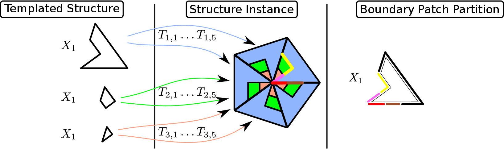
On the right the boundary patch partition of the template $X_1$ is visualized. The boundary patch partition elements colored in red and brown are not obvious when viewing only a single slice. These boundary patch partition elements are indicated by the neighboring instances in other slices.

Like with reflective symmetries, a multi-region geometry or multi-region mesh is said to have a rotational symmetry, if every region has the same rotational symmetry. For a multi-region geometry (or multi-region mesh) with a rotational symmetry of order $n$, a region might also have a rotational symmetry with the same rotation center and rotation axis but rotational symmetry order of $k$, where $n$ is a factor of $k$. As for reflective meshes, the templated structure of a multi-region geometry or mesh has one template for each region. However, the boundary patch partition for each template (which represents a region) might be more complex than described above (cf. Figure 6.8). The instance graph, however, is still regular, because no new transformation functions are introduced.

Any mesh generation algorithm presented in Section 5.1 can be used to create a templated mesh based on a multi-region geometry with a rotational symmetry. Due to the simple structure of a rotationally symmetric object, the calculation of the boundary patch partition can be simplified as described in Algorithm 6.2.

At first, the slice with a starting angle of $\sigma$ is calculated (Line 5). One half of the first hyperplane of this slice (with starting angle $\sigma$) is explicitly obtained (Line 6-7). Using this half hyperplane, a manifold partition for all regions is obtained, where the region is intersected with the half hyperplane (Line 10). These manifold partitions are refined (Line 11) and rotated (Line 13) to the other hyperplane of the slice to obtain a manifold partition of the slice hyperplanes $B_S$. Then, for each region, the section which lies within the slice is obtained (Line 15). The boundary patch partition of the region slice is calculated by using all elements of $B_S$, which are included in the region (Line 16) and the complement of the region slice boundary (Line 17). Although Algorithm 6.2 is formulated for 3D multi-region geometries, it can also be applied to 2D geometries. In that case, the rotation axis $v$ is not needed and the hyperplane and slice creation as well as the rotation functions are less complicated to calculate.

In contrast to reflective symmetries, rotational symmetries promise higher improvements in memory and mesh generation runtime. Assuming no overhead, a theoretical improvement of a factor of $n$ could be achieved for geometries with rotational symmetry of order $n$ (in contrast to an improvement of two for reflective symmetries).

However, one issue with rotational symmetries is the appearance of small angles for objects with a high rotational symmetry order. In particular, a slice of a set $A$ with a rotational symmetry of order $n$ and the rotation center (as well as a neighborhood) included in $A$ has an internal angle equal to $\alpha = 360\degree/n$ at the rotation center. For large $n$, this angle can be very small and therefore an issue for mesh generation processes, especially for algorithms with guaranteed mesh element qualities, like mesh generation algorithms based on Delaunay refinement (cf. Section 3.1.1). A possible solution for issues with small angles is given in Section 6.3.2.