Finding Optimal Slicing Positions

**Figure 6.9:** Examples for possible slice positions
$\begin{subfigure} % latex2html id marker 12389 [t]{0.35\textwidth} \centering ... ...{figures/slicing_position_good} \caption{\emph{Good} position} \end{subfigure}$ $\begin{subfigure} % latex2html id marker 12396 [t]{0.35\textwidth} \centering ... ...h]{figures/slicing_position_bad} \caption{\emph{Bad} position} \end{subfigure}$ While the slice position shown in (top picture) introduces a small inner angle (visualized in red) which potentially affects the mesh element quality in a negative way, the slice position shown in (bottom picture) is optimal, meaning that the newly introduced angles are minimized.

The choice of the starting angle $\sigma$ of a slice has a potential impact on the mesh element quality as some slice positions might introduce small inner angles as visualized in Figure 6.9. It is therefore of interest to find an optimal starting angle for the slice. Because of the periodicity with respect to the angles, it is sufficient to only check and analyze starting angles $\sigma$ in the range of $[0, \alpha)$ .

**Figure 6.10:** Piecewise linear slice starting angle
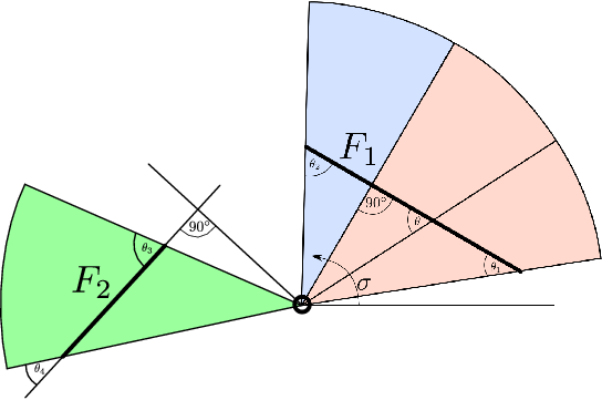
The newly introduced angle $\theta$ between and and a potential slice hyperplane is piecewise linearly dependent on the slice hyperplane angle $\sigma$ . In the red section, $\theta$ starts at the angle $\theta_1$ and increases linearly to a maximum of $90\degree$ and in the blue section, the angle $\theta$ starts at a maximum of $90\degree$ and decreases linearly to $\theta_2$ . Because the closest point of the affine hull of facet is not included in , there is only one section (colored in green), where $\theta$ starts at a maximum angle of $\theta_3$ and decreases linearly to $\theta_4$ .

For linear geometries (using boundary representation), Algorithm 6.3 evaluates all possible slice positions and returns a slice position which maximizes the smallest, newly introduced inner angle. For each facet which is intersected by a slice hyperplane, a new angle $\theta$ between that facet and the hyperplane is introduced. This angle $\theta$ is (piecewise) linearly dependent on the starting angle $\sigma$ as shown in Figure 6.10. The algorithm partitions the slice starting angle interval $[0, \alpha)$ into sections where for every facet the angle between a potential slice hyperplane and facet is linear.

Then, for each of these sections a linear optimization is used to maximize the smallest newly introduced angle. The section with the largest newly introduced angle is chosen as the optimal slice position.

Algorithm 6.3 is formulated for 3D linear geometries but also works for 2D linear geometries with some minor modifications. For simplicity, the input geometry is assumed to have its center located at the origin and the z-axis is the rotation axis. At first, all facets which are (partially) included in a slice with a starting angle of zero and spanning angle of $\alpha$ are obtained (Line 5). The section, for which the newly introduced angles for every facet are linear, is stored in which is initially set to the angle interval $[0, \alpha)$ (Line 6). For each vertex of a facet, the angle of that vertex (in relation to the center and the x-axis) is calculated and sorted in ascending order (Lines 8-12).

If the first and the last angle are equal, than the facet is radial and no additional angles are introduced between that facet and any potential slice hyperplane (Line 13). The angle of the first vertex $\theta[1]$ and the angle of the last vertex $\theta[k]$ are new separation points for the sections in and therefore added to (Line 16). In Lines 17 to 21, the angle (to the x-axis) of the closest point of the facet (to the origin) is also added to , if that angle is in the interval $[\theta[1], \theta[k]]$ (cf. Figure 6.10 for an explanation why this is required). The section separation points in are then sorted in ascending order (Line 24) and for every two consecutive elements of , an interval is formed. The angle of a potential slice hyperplane and every facet is linear in that interval. Therefore, a linear optimization is used to find the slice hyperplane angle $\tilde{\sigma}$ which maximizes the smallest newly introduced angle (Line 29). If this maximal smallest angle $\tilde{\sigma}$ is larger than any previous best choice $\sigma$ , $\tilde{\sigma}$ is used as a new best choice (lines 30-34).

6.3.1 Finding Optimal Slicing Positions