7.5 FEM-based Symmetry Analysis using a Five-pointed Star

Figure 7.13: The Gummel Star with non-symmetric boundary conditions

\begin{subfigure}
% latex2html id marker 16298
[b]{0.25\textwidth}
\centering
...
...onsymemtric_boundary_conditions}
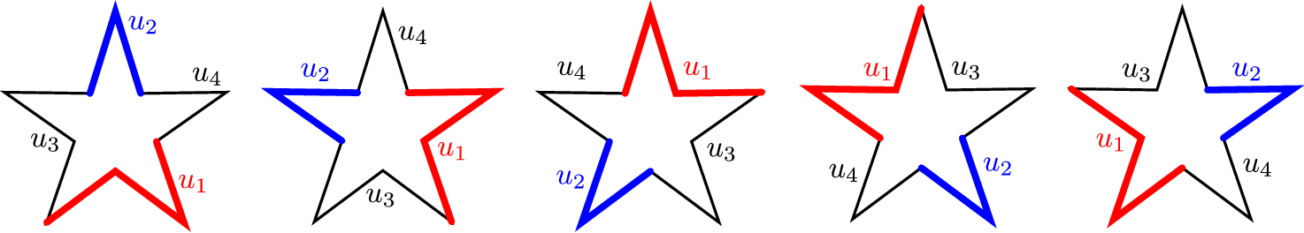
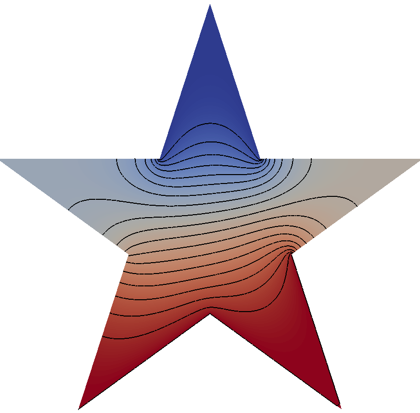
\caption{Boundary conditions}
\end{subfigure} \begin{subfigure}
% latex2html id marker 16310
[b]{0.45\textwidth}
\centering
...
...itions_dual}
\caption{Boundary conditions of the dual problem}
\end{subfigure}

Boundaries colored in red and blue are Dirichlet boundaries with constant value $ {\color{red}u_1} = 1$ and $ {\color{blue}u_2} = 0$, respectively. The remaining boundaries $ u_2$ and $ u_3$ are Neumann boundaries. The solution to that boundary value problem is visualized in the middle. The boundary conditions of the dual problem are visualized on the right.

An investigation of the effects of the templated approach on the solution of a simulation problem with symmetric geometry is presented in this section. In particular, a boundary value problem based on the Laplace equation [57] is investigated on a symmetric five-pointed star. This simulation problem, visualized in Figure 7.13, is referred to as Gummel Star [126] and has the following two interesting properties: First, due to the rotational symmetry of the simulation domain, rotating the boundary conditions results in a solution which is equal to the rotated solution of the initial problem. Second, the dual problem - the simulation problem where the Dirichlet and the Neumann boundaries are swapped (cf. Figure 7.13c) - is equal to the reflected simulation problem, hence resulting in a solution which is equal to the reflected solution of the initial problem. However, as stated in Chapter 1, these two properties might not hold for numerical solutions when using non-symmetric meshes.

Figure 7.14: Non-symmetric and symmetric example meshes of the Gummel Star

Figure 7.15: All rotations of the non-symmetric Gummel Star boundaries
Image gummel_star_boundary_rotations

To investigate the effects on the numerical solution, three types of meshes have been generated for different target cell sizes: a non-symmetric, a rotationally symmetric, and a reflective-rotationally symmetric mesh. All meshes have been created with a smallest angle quality larger than $ 30 \degree$ [109]. Example meshes for each type are visualized in Figure 7.14. For each mesh and each rotation of the boundary conditions (cf. Figure 7.15), solutions to the boundary value problem as well as the dual boundary value problem have been calculated using the free open source FEM software framework FEniCS [4]. These solutions are compared by first rotating (for the rotated boundary conditions) or reflecting (for the dual problem) them to be aligned and then applying the maximum norm on the transformed solutions. The solution difference of two solutions $ u$ and $ v$ is therefore defined as:

$\displaystyle d(u,v) := \max_{x \in D} \left\lVert u(x) - v(T(x)) \right\rVert_{\infty} = \max_{x \in D} \left\vert u(c) - v(T(x)) \right\vert$ (7.1)

$ D$ is the simulation domain and $ T$ is the transformation which aligns the solution $ v$ to the solution $ u$. It is to be expected that meshes with rotational symmetries yield numerically equal solutions when rotating the boundary conditions. Additionally, meshes with reflective symmetries are expected to yield numerically equal solutions when comparing the initial problem to the dual problem.

The solution differences for the rotated boundary conditions on meshes with two different cell counts are given in Table 7.2 and Table 7.3. Each row and each column represents the solution to the boundary value problem with rotated boundary conditions. The differences on the non-symmetric meshes are at least two orders of magnitude, for the coarser meshes (cf. Table 7.2) even three orders of magnitude, larger then the differences on the symmetric meshes. Additionally, keeping in mind that the largest value of the solution to this boundary value problem is one, the errors for the non-symmetric mesh range up to $ 11\%$.


Table 7.2: Solution differences for the rotated boundary conditions on meshes with about $ 1.2 \times 10^2$ triangles. All solution differences are evaluated by rotating the solutions to a position where they are aligned and then applying the maximum norm. The solution differences for the non-symmetric mesh are at least three orders of magnitude larger than the solution differences for the rotationally and the reflective-rotationally symmetric mesh. The solution differences for the rotationally and reflective-rotationally symmetric mesh are not exactly zero due to numeric issues and round-off errors. However, these differences indicate that these solutions are numerically equal.

No rotation 72° rotation 144° rotation 216° rotation 288° rotation
Non-symmetric mesh with $ 109$ triangles
No rotation $ \color{OliveGreen} 0$ $ \color{red} 5.0 \times 10^{-2\phantom{0}}$ $ \color{red} 1.1 \times 10^{-1\phantom{0}}$ $ \color{red} 7.2 \times 10^{-2\phantom{0}}$ $ \color{red} 4.2 \times 10^{-2\phantom{0}}$
Rotation $ 72\degree$ $ \color{OliveGreen} 0$ $ \color{red} 1.1 \times 10^{-1\phantom{0}}$ $ \color{red} 7.0 \times 10^{-2\phantom{0}}$ $ \color{red} 5.6 \times 10^{-2\phantom{0}}$
Rotation $ 144\degree$ $ \color{OliveGreen} 0$ $ \color{red} 1.1 \times 10^{-1\phantom{0}}$ $ \color{red} 1.1 \times 10^{-1\phantom{0}}$
Rotation $ 216\degree$ $ \color{OliveGreen} 0$ $ \color{red} 1.0 \times 10^{-1\phantom{0}}$
Rotation $ 288\degree$ $ \color{OliveGreen} 0$
Rotationally symmetric mesh with $ 120$ triangles
No rotation $ \color{OliveGreen} 0$ $ 1.1 \times 10^{-5\phantom{0}}$ $ 9.8 \times 10^{-6\phantom{0}}$ $ 6.1 \times 10^{-6\phantom{0}}$ $ 8.4 \times 10^{-6\phantom{0}}$
Rotation $ 72\degree$ $ \color{OliveGreen} 0$ $ 1.2 \times 10^{-5\phantom{0}}$ $ 6.7 \times 10^{-6\phantom{0}}$ $ 9.7 \times 10^{-6\phantom{0}}$
Rotation $ 144\degree$ $ \color{OliveGreen} 0$ $ 7.4 \times 10^{-6\phantom{0}}$ $ 6.6 \times 10^{-6\phantom{0}}$
Rotation $ 216\degree$ $ \color{OliveGreen} 0$ $ 8.4 \times 10^{-6\phantom{0}}$
Rotation $ 288\degree$ $ \color{OliveGreen} 0$
Reflective-rotationally symmetric mesh with $ 130$ triangles
No rotation $ \color{OliveGreen} 0$ $ 1.6 \times 10^{-5\phantom{0}}$ $ 1.2 \times 10^{-5\phantom{0}}$ $ 9.4 \times 10^{-6\phantom{0}}$ $ 1.6 \times 10^{-5\phantom{0}}$
Rotation $ 72\degree$ $ \color{OliveGreen} 0$ $ 1.6 \times 10^{-5\phantom{0}}$ $ 1.0 \times 10^{-5\phantom{0}}$ $ 1.2 \times 10^{-5\phantom{0}}$
Rotation $ 144\degree$ $ \color{OliveGreen} 0$ $ 8.5 \times 10^{-6\phantom{0}}$ $ 1.0 \times 10^{-5\phantom{0}}$
Rotation $ 216\degree$ $ \color{OliveGreen} 0$ $ 1.6 \times 10^{-5\phantom{0}}$
Rotation $ 288\degree$ $ \color{OliveGreen} 0$


Table 7.3: Solution differences for the rotated boundary conditions on meshes with about $ 1.4 \times 10 ^ 4$ triangles. All solution differences are evaluated by rotating the solutions to a position where they are aligned and then applying the maximum norm. The solution differences for the non-symmetric mesh are at least two orders of magnitude larger than the solution differences for the rotationally and the reflective-rotationally symmetric mesh. The solution differences for the rotationally and reflective-rotationally symmetric mesh are not exactly zero due to numeric issues and round-off errors. However, these differences indicate that these solutions are numerically equal.

No rotation 72° rotation 144° rotation 216° rotation 288° rotation
Non-symmetric mesh with $ 13921$ triangles
No rotation $ \color{OliveGreen} 0$ $ \color{red} 1.1 \times 10^{-2\phantom{0}}$ $ \color{red} 2.5 \times 10^{-2\phantom{0}}$ $ \color{red} 3.5 \times 10^{-2\phantom{0}}$ $ \color{red} 1.9 \times 10^{-2\phantom{0}}$
Rotation $ 72\degree$ $ \color{OliveGreen} 0$ $ \color{red} 2.5 \times 10^{-2\phantom{0}}$ $ \color{red} 3.5 \times 10^{-2\phantom{0}}$ $ \color{red} 1.9 \times 10^{-2\phantom{0}}$
Rotation $ 144\degree$ $ \color{OliveGreen} 0$ $ \color{red} 1.3 \times 10^{-2\phantom{0}}$ $ \color{red} 1.5 \times 10^{-2\phantom{0}}$
Rotation $ 216\degree$ $ \color{OliveGreen} 0$ $ \color{red} 2.2 \times 10^{-2\phantom{0}}$
Rotation $ 288\degree$ $ \color{OliveGreen} 0$
Rotationally symmetric mesh with $ 13850$ triangles
No rotation $ \color{OliveGreen} 0$ $ 9.2 \times 10^{-5\phantom{0}}$ $ 8.0 \times 10^{-5\phantom{0}}$ $ 7.7 \times 10^{-5\phantom{0}}$ $ 9.2 \times 10^{-5\phantom{0}}$
Rotation $ 72\degree$ $ \color{OliveGreen} 0$ $ 8.4 \times 10^{-5\phantom{0}}$ $ 7.7 \times 10^{-5\phantom{0}}$ $ 8.0 \times 10^{-5\phantom{0}}$
Rotation $ 144\degree$ $ \color{OliveGreen} 0$ $ 7.9 \times 10^{-5\phantom{0}}$ $ 8.0 \times 10^{-5\phantom{0}}$
Rotation $ 216\degree$ $ \color{OliveGreen} 0$ $ 8.9 \times 10^{-5\phantom{0}}$
Rotation $ 288\degree$ $ \color{OliveGreen} 0$
Reflective-rotationally symmetric mesh with $ 14160$ triangles
No rotation $ \color{OliveGreen} 0$ $ 1.1 \times 10^{-4\phantom{0}}$ $ 1.3 \times 10^{-4\phantom{0}}$ $ 9.5 \times 10^{-5\phantom{0}}$ $ 1.1 \times 10^{-4\phantom{0}}$
Rotation $ 72\degree$ $ \color{OliveGreen} 0$ $ 9.9 \times 10^{-5\phantom{0}}$ $ 8.0 \times 10^{-5\phantom{0}}$ $ 1.3 \times 10^{-4\phantom{0}}$
Rotation $ 144\degree$ $ \color{OliveGreen} 0$ $ 7.9 \times 10^{-5\phantom{0}}$ $ 8.0 \times 10^{-5\phantom{0}}$
Rotation $ 216\degree$ $ \color{OliveGreen} 0$ $ 9.9 \times 10^{-5\phantom{0}}$
Rotation $ 288\degree$ $ \color{OliveGreen} 0$


The solution differences for the initial and the dual problem for meshes with different cell counts are given in Table 7.4. The solution differences are at least two orders of magnitude smaller when using a reflective-rotationally symmetric mesh compared to a non-symmetric mesh. Additionally, due to the lack of reflective symmetry, the solution differences for the rotationally symmetric mesh are about one order of magnitude larger than the differences for the reflective-rotationally symmetric mesh.


Table 7.4: Solution differences of the initial problem and its dual problem for meshes with different symmetries and cell counts. Solution differences are evaluated by reflecting the dual solution to make it aligned to the solution of the initial problem and then applying the maximum norm. As expected, the differences for the reflective-rotationally mesh are always less then the differences for the non-symmetric or the rotationally symmetric mesh. However, the rotationally symmetric meshes yields solutions which are more similar than the solutions for the non-symmetric mesh.

Symmetry type Cell count Solution difference using the maximum norm
Non-symmetric $ 109$ $ \color{red} 5.0 \times 10^{-2\phantom{0}}$
Rotationally symmetric $ 120$ $ \color{red} 1.4 \times 10^{-2\phantom{0}}$
Reflective-rotationally symmetric $ 130$ $ 1.6 \times 10^{-5\phantom{0}}$
Non-symmetric $ 1758$ $ \color{red} 2.4 \times 10^{-2\phantom{0}}$
Rotationally symmetric $ 1740$ $ 3.2 \times 10^{-3\phantom{0}}$
Reflective-rotationally symmetric $ 1750$ $ 6.5 \times 10^{-5\phantom{0}}$
Non-symmetric $ 13921$ $ \color{red} 1.2 \times 10^{-2\phantom{0}}$
Rotationally symmetric $ 13850$ $ 1.1 \times 10^{-3\phantom{0}}$
Reflective-rotationally symmetric $ 14160$ $ 1.1 \times 10^{-4\phantom{0}}$
Non-symmetric $ 111244$ $ \color{red} 1.2 \times 10^{-2\phantom{0}}$
Rotationally symmetric $ 111260$ $ 1.1 \times 10^{-3\phantom{0}}$
Reflective-rotationally symmetric $ 111660$ $ 2.8 \times 10^{-4\phantom{0}}$


As expected, meshes with rotational symmetries yield solutions which are (numerically) equal to each other when rotating the boundary conditions of the Gummel star. Also, meshes with reflective symmetries yield solutions to the initial and the dual problem which are, again, numerically equal.

florian 2016-11-21