|
|
|
|
Previous: 4.4.1.2 Normalization of the Stationary Distribution Function Up: 4.4.1 Solution of the Zeroth Order Equation Next: 4.4.2 Solution of the First Order Equation |
|
|
|
|
Previous: 4.4.1.2 Normalization of the Stationary Distribution Function Up: 4.4.1 Solution of the Zeroth Order Equation Next: 4.4.2 Solution of the First Order Equation |
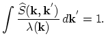
Further, an additional differential scattering rate
![]() is introduced
is introduced
 |
(4.67) |
Now taking into account (4.65) and (4.67) the scattering operator (4.64) takes the conventional form:
![$\displaystyle Q[f_{s}]=\int f_{s}(\vec{k}^{'})\widehat{S}(\vec{k}^{'},\vec{k})\,d\vec{k}^{'}-f_{s}(\vec{k})\lambda(\vec{k}).$](img1037.png) |
(4.68) |
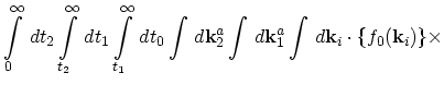
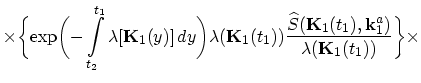
Using the Neumann series of the forward equation the second iteration term (4.47) is derived as an example:
Within the algorithm presented in [82] the before-scattering distribution function is equal to
![]() which gives the distribution
which gives the distribution ![]() . In order to find the distribution function of the
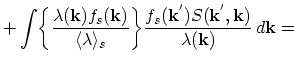
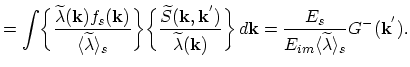
after-scattering states the before-scattering distribution function should be multiplied by the conditional probability density for an after-scattering
state and this product is integrated over all before-scattering states. Using (4.67) and (4.66) one obtains for the
after-scattering distribution:
. In order to find the distribution function of the
after-scattering states the before-scattering distribution function should be multiplied by the conditional probability density for an after-scattering
state and this product is integrated over all before-scattering states. Using (4.67) and (4.66) one obtains for the
after-scattering distribution:
![$\displaystyle \int\biggl\{\frac{\lambda(\vec{k})f_{s}(\vec{k})}{\langle\lambda\...
...frac{[1-f_{s}(\vec{k}^{'})]S(\vec{k},\vec{k}^{'})}{\lambda(\vec{k})}\,d\vec{k}+$](img1047.png) |
|||
![$\displaystyle +\frac{\lambda(\vec{k}^{'})f_{s}(\vec{k}^{'})}{\langle\lambda\ran...
...frac{[1-f_{s}(\vec{k}^{'})]S(\vec{k},\vec{k}^{'})}{\lambda(\vec{k})}\,d\vec{k}+$](img1048.png) |
(4.70) | ||
 |
|||
 |
S. Smirnov:
![$\displaystyle [1-f_{s}(\vec{k})]\int f_{s}(\vec{k}^{'})S(\vec{k}^{'},\vec{k})\,...
...lpha(\vec{k}^{'})\lambda(\vec{k}^{'})\delta(\vec{k}-\vec{k}^{'})\,d\vec{k}^{'}-$](img1029.png)
![$\displaystyle -f_{s}(\vec{k})\biggl\{\int[1-f_{s}(\vec{k}^{'})]S(\vec{k},\vec{k}^{'})\,d\vec{k}^{'}+\alpha(\vec{k})\lambda(\vec{k})\biggr\},$](img1030.png)
![$\displaystyle \lambda(\vec{k})=\int[1-f_{s}(\vec{k}^{'})]S(\vec{k},\vec{k}^{'})\,d\vec{k}^{'}+\alpha(\vec{k})\lambda(\vec{k}).$](img1032.png)
![$\displaystyle \times\biggl\{\exp\biggl(-\int_{0}^{t_{2}}\lambda[\vec{K}_{2}(y)]...
...\vec{K}_{2}(t_{2}),\vec{k}_{2}^{a})}{\lambda(\vec{K}_{2}(t_{2}))}\biggr\}\times$](img1040.png)
![$\displaystyle \times\biggl\{\exp\biggl(-\int_{t_{1}}^{t_{0}}\lambda[\vec{K}(y)]...
...c{K}(t_{0}))\biggr\}
\Theta(t-t_{1})\Theta_{\Omega}(\vec{K}(t))\Theta(t_{0}-t).$](img1042.png)