Next: 3. 2. 5 Volume Integration Up: 3. 2 Finite Volume Schemes Previous: 3. 2. 3 Topological Structure of the
One method typically used in simulation is the dual graph method. As an introductory example, the numerical solution of the Laplace equation is shown. In this case the functional ![]() is the gradient and
is the gradient and ![]() .
.
For linear shape functions, the function
![]() along one edge can be written as
along one edge can be written as
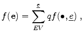 |
(3.34) |
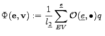 |
(3.35) |
![$\displaystyle R = [m\mathcal{L}f] = \sum_{VE}^{\underline{v}} \mathcal{O}(\bull...
...frac{A}{l} \sum_{EV}^{\underline{e}} \mathcal{O}(\underline{e}, \bullet) q \; .$](img313.png) |
(3.36) |
![\includegraphics[width=10cm]{DRAWINGS/fvm_topo.eps}](img304.png)