4. 1. 6 Example - Nonlinear Conductivity

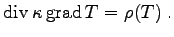
In the following section it is assumed that the thermal capacitance $\rho$ depends on the temperature of the respective material. In analogy a nonlinear dependence of the thermal conductance $\kappa$ with respect to the temperature can be specified. However, for the sake of simplicity the heat conductance $\kappa$ is assumed to be constant in the following example.

$$\mathrm{div} \, \kappa \, \mathrm{grad} \, T = \rho(T) \; .$$ (4.18)

A finite volume discretization yields for the same four-point geometry as in the linear example of the last section:

$$R := \sum_{VNV}^{\underline{v}} \kappa Q K(\bullet, \underline{v}) - \rho(Q)$$

By inserting the neighborhood information and setting the thermal generation term $q=1$ and $\rho(q)= q^2$ , the following expression is obtained.

$$R(\mathbf{v}_1) := -2 Q(\mathbf{v}_1) + Q(\mathbf{v}_2) -\rho_0 Q(\mathbf{v}_1)^2$$

$$R(\mathbf{v}_2) := -2 Q(\mathbf{v}_2) + Q(\mathbf{v}_1) -\rho_0 (\mathbf{v}_2)^2$$ (4.19)

When using the Newton method it is always assumed that a given (already good) result is used to obtain a better result (see Fig. ). For the linear problem, a Newton scheme leads to a solution within one single step, because all higher-order terms vanish. For this reason in the linear case the choice of an initial guess does not play a role.

Figure: The solutions of the linearized problems converge to the solution of the nonlinear problem using the Newton method.

For the nonlinear case, it is however important to chose a proper initial guess. In the following, the initial values $q(\mathbf{v}_1) = q(\mathbf{v}_2) = -0.2$ is chosen. Therefore, the expressions $Q(\mathbf{v}_1)$ and $Q(\mathbf{v}_2)$ yield

$$Q(\mathbf{v}_1) := [1, 0; -0.2]$$

$$Q(\mathbf{v}_2) := [0, 1; -0.2]$$ (4.20)

First, the application of the $\rho_0 Q(\mathbf{v}_1) \cdot Q(\mathbf{v}_1)$ is performed as follows

$$Q(\mathbf{v}_1) \cdot T_1 = [1, 0; -0.2] \cdot [1, 0; -0.2] =$$

$$Q(\mathbf{v}_1) \cdot [-0.4, 0; 0.04] = \cdot [-0.4, 0; 0.04]$$ (4.21)

Repeated application of this step (eventually) leads to a solution of this equation system. However, it has to be considered that nonlinear methods have different rates of convergence and sometimes solutions can not be found at all [82]. Nevertheless, the presented method with linearized expressions can be used for the formulation of all kinds of nonlinear problems, the solution of these problems can be treated separately from the assembly.