4. 1. 9 Eigenvalue Problems

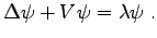
The use of linearized expressions can also be generalized so as to be employed for the specification of eigenvalue equations. In this case, expressions of the form $\mathbf{A} \mathbf{x} = \lambda \mathbf{B} \mathbf{x}$ the linearized expression can be specified. The Schrödinger equation which is typically used for the solution of quantum mechanical problems is a basic example for the treatment of eigenvalue equations using linear expressions.

Figure4.3: The eigenvalue problem is specified on a four point one-dimensional equi-distant domain, where the two boundary points are set to zero. Two eigenvectors are shown.

$$\Delta \psi + V \psi = \lambda \psi \; .$$ (4.25)

The eigenvalue equation system can be written in the following line-wise form:

$$\mathcal{E}_k = \sum_i c_{i, k} v_i + \lambda \sum_j d_{j, k} v_j (=0) \; .$$ (4.26)

For the sake of simplicity and in order to obtain a consistent short and concise notation comparable to linearized expressions (4.9), the following scheme is introduced:

$$\sum_i c_i v_i + \lambda \sum_j d_j v_j =: [c_1, \ldots, c_N ; d_1, \ldots, d_N ]$$ (4.27)

As these eigenvalue equations are always linear, only linear operations have to be considered and a linear space is obtained.

$$[c_1, \ldots, c_N ; d_1, \ldots, d_N ] + [e_1, \ldots, e_N ; f_1, \ldots, f_N ] =$$

$$[c_1+e_1, \ldots, c_N+e_N ; d_1+f_1, \ldots, d_N+f_N ]$$ (4.28)

$$[c_1, \ldots, c_N ; d_1, \ldots, d_N ] - [e_1, \ldots, e_N ; f_1, \ldots, f_N ] =$$

$$[c_1-e_1, \ldots, c_N-e_N ; d_1-f_1, \ldots, d_N-f_N ]$$ (4.29)

$$a \cdot [c_1, \ldots, c_N ; d_1, \ldots, d_N ] =$$

$$[a \cdot c_1, \ldots, a \cdot c_N ; a \cdot d_1, \ldots, a \cdot d_N ]$$ (4.30)

$$\lambda([c_1, \ldots, c_N ; 0, \ldots, 0 ]) = [0, \ldots, 0 ; c_1, \ldots, c_N ]$$ (4.31)

An algebraic structure which introduces linear(ized) expressions to eigenvalue- expressions has to provide the following elements:

$$\mathrm{hom}([c_1, \ldots, c_N ; q]) = [c_1, \ldots, c_N ; 0, \ldots, 0 ]$$ (4.32)

$$\lambda([c_1, \ldots, c_N ; q]) = [0, \ldots, 0 ; c_1, \ldots, c_N ]$$ (4.33)

The following discretization is obtained in a one-dimensional simulation domain according to Figure 4.1 comprising four vertices when using finite differences. The solution is referred to as $\psi$ which is stored in the quantity $q$ . In analogy to (4.12), the term $Q$ is introduced.

$$R(\mathbf{v}_1) = -2 Q(\mathbf{v}_1) + Q(\mathbf{v}_2) + V(\mathbf{v}_1) Q(\mathbf{v}_1) - \lambda Q(\mathbf{v}_1) = 0\;$$

$$R(\mathbf{v}_2) = -2 Q(\mathbf{v}_2) + Q(\mathbf{v}_1) + V(\mathbf{v}_2) Q(\mathbf{v}_2) - \lambda Q(\mathbf{v}_2) = 0 \; .$$ (4.34)

The potential is assigned constant values 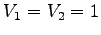$V_1 = V_2 = 1$ . For the probability function $\psi_i$ the following term is inserted

$$Q(\mathbf{v}_1) = [1, 0; 0, 0]$$

$$Q(\mathbf{v}_2) = [0, 1; 0, 0] \; .$$ (4.35)

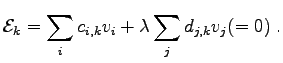
Accordingly, one obtains the following eigenvalue expressions:

$$R(\mathbf{v}_1) = -2 [1, 0; 0, 0] + [0, 1; 0, 0] + [1, 0; 0, 0] - \lambda [1, 0; 0, 0] \;$$

$$R(\mathbf{v}_1) = [-1, 1; 1, 0]$$

$$R(\mathbf{v}_2) = [1, -1; 0, 1]$$ (4.36)

In analogy to linearized expressions, linear eigenvalue expressions can be used in order to fill the eigenvalue matrices. One often observes that the matrix $B$ is the unit matrix. Often it is necessary to change the order of the equations in order to maintain the unit matrix for $B$ .