Surface Roughness Scattering

The deviations of the interface from an ideal flat plane can be described by a two-dimensional roughness fluctuation, $\Delta({\ensuremath{\mathitbf{r}}})$, where $\mathitbf{r}$ is the two-dimensional position vector in the plane of the interface [Ferry97]. The potential associated with the roughness $\Delta({\ensuremath{\mathitbf{r}}})$ can be viewed as a combination of two effects:

• The boundary perturbation causes the envelope functions to be displaced from their unperturbed positions.
• The imposed fluctuation of the electric field and the charge density at the rough interface give rise to an electrostatic contribution to the potential.

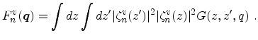
The original formulation of Prange and Nee [Prange68] of the unscreened matrix elements for surface roughness scattering has been adopted. It can be applied for scattering at two interfaces [Esseni04]

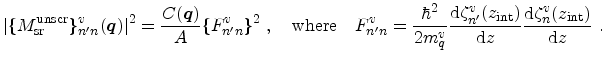$$\vert\{M^\mathrm{unscr}_\mathrm{sr} \}_{n'n}^v({\ensuremath{\math... ...{int})}{\mathrm{d}z} \frac{\mathrm{d}\zeta_n^v(z_\mathrm{int})}{\mathrm{d}z}\ .$$ (5.31)

Here, ${\ensuremath{\mathitbf{q}}} = {\ensuremath{\mathitbf{k}}} - {\ensuremath{\mathitbf{k}}}'$ is the momentum transfer, $m_{q}^v$ is the quantization mass of electrons in valley $v$, and $\mathrm{d}\zeta_n^v(z_\mathrm{int})/\mathrm{d}z$ denotes the derivative of the envelope function with respect to $z$ at the position of the interface (for instance, $z_\mathrm{int}=0$, and $z_\mathrm{int}=T_{\mathrm{si}}$ for the front and back-interface of a thin Si film). The spectral density $C({\ensuremath{\mathitbf{q}}})$ is the 2D Fourier transform of the autocovariance function

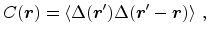$$C({\ensuremath{\mathitbf{r}}}) = \langle \Delta({\ensuremath{\mat... ...) \Delta({\ensuremath{\mathitbf{r}}}' - {\ensuremath{\mathitbf{r}}}) \rangle\ ,$$ (5.32)

where the brackets denote the ensemble average of the roughness fluctuation $\Delta({\ensuremath{\mathitbf{r}}})$. The roughness spectrum is frequently assumed to be Gaussian [Jungemann93,Esseni03,Esseni04]

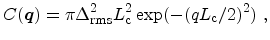$$C({\ensuremath{\mathitbf{q}}}) = \pi \ensuremath {\Delta_\mathrm{rms}}^2\ensuremath {L_\mathrm{c}}^2 \exp(-(q\ensuremath {L_\mathrm{c}}/2)^2)\ ,$$ (5.33)

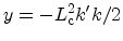
or of exponential shape [Goodnick85,Ferry97]

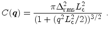$$C({\ensuremath{\mathitbf{q}}}) = \frac{\pi \ensuremath {\Delta_\m... ...nsuremath {L_\mathrm{c}}^2}{(1+(q^2\ensuremath {L_\mathrm{c}}^2 / 2))^{3/2}}\ .$$ (5.34)

Here, is the root mean square value of the roughness fluctuations and is the autocovariance length.

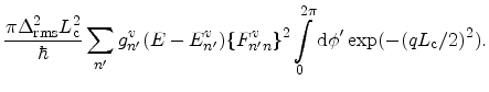
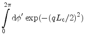
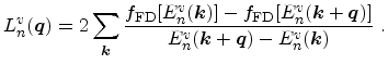
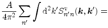
The transition rate for surface roughness scattering is

$$S_{n'n}^{v} ({\ensuremath{\mathitbf{k}}}, {\ensuremath{\mathitbf{... ...'}^{v}({\ensuremath{\mathitbf{k}}}') - E_n^{v}({\ensuremath{\mathitbf{k}}})]\ ,$$ (5.35)

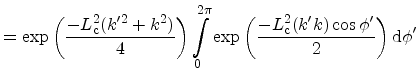
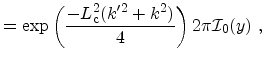
where intersubband transitions due to surface roughness are restricted to the same valley [Esseni03,Cheng71]. In the nonparabolic band approximation the scattering rate for a Gaussian spectrum is given by

$$\frac{A}{4\pi^2} \sum_{n'} \int \mathrm{d}^2 k' S_{n'n}^{v} ({\ensuremath{\mathitbf{k}}}, {\ensuremath{\mathitbf{k}}}') =$$

$$\frac{\ensuremath {\Delta_\mathrm{rms}}^2\ensuremath {L_\mathrm{c... ...n'}^{v}({\ensuremath{\mathitbf{k}}}') - E_n^{v}({\ensuremath{\mathitbf{k}}})] =$$

$$\frac{\pi \ensuremath {\Delta_\mathrm{rms}}^2\ensuremath {L_\math... ...}^v\}^2 \int_0^{2\pi} \mathrm{d}\phi' \exp(-(q\ensuremath {L_\mathrm{c}}/2)^2).$$ (5.36)

Assuming isotropic bands $m^{v} = m^v_{\shortparallel,1} \approx m^v_{\shortparallel,2} \approx \sqrt{m_{\shortparallel,1} m_{\shortparallel,2}}$, the integral over the angle can be written as

$$\int_0^{2\pi} \mathrm{d}\phi' \exp(-(q\ensuremath {L_\mathrm{c}}/2)^2) = \exp\left( \frac{-\ensuremath {L_\mathrm{c}}^2(k'^2 + k^2)}{4} ... ...frac{-\ensuremath {L_\mathrm{c}}^2(k'k)\cos \phi' }{2} \right ) \mathrm{d}\phi'$$

$$= \exp\left( \frac{-\ensuremath {L_\mathrm{c}}^2(k'^2 + k^2)}{4} \right ) 2\pi \mathcal{I}_0(y)\ ,$$ (5.37)

where $y = -\ensuremath {L_\mathrm{c}}^2k'k/2$, and $\mathcal{I}_0$ denotes the modified Bessel function of the first kind.

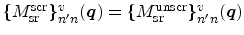
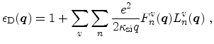
Since the electrons in the inversion layer screen the scattering potential, the transition rate for surface roughness scattering is reduced. The dielectric function relates the unscreened and screened matrix elements of the scattering potential through the dielectric function $\ensuremath {\epsilon_\mathrm{D}}{}$

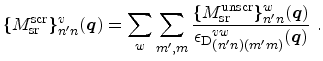$$\{M^\mathrm{scr}_\mathrm{sr} \}_{n'n}^v({\ensuremath{\mathitbf{q}... ...math {\epsilon_\mathrm{D}}{}_{(n'n)(m'm)}^{vw}({\ensuremath{\mathitbf{q}}})}\ .$$ (5.38)

Because surface roughness represents a static potential the dependence on the frequency $\omega$ can be dropped. Since the number of relevant subbands can be of order 100 [Jungemann93], further simplifications are required to numerically evaluate the impact of screening.

In the long-wavelength limit, ${\ensuremath{\mathitbf{q}}} \rightarrow 0$, intersubband transitions are completely unscreened [Ferry97], thus $\{M^\mathrm{scr}_\mathrm{sr} \}_{n'n}^v({\ensuremath{\mathitbf{q}}}) = \{M^\mathrm{unscr}_\mathrm{sr} \}_{n'n}^v({\ensuremath{\mathitbf{q}}})$. Furthermore, the multisubband dielectric function reduces to a scalar function when neglecting the intersubband polarizabilities and the correction terms due to the intrasubband polarizabilities of the other subbands [Ferry97]. This approximation is frequently applied for transport simulations [Esseni03,Esseni04]. The scalar dielectric function for intrasubband transitions can be given in terms of the polarization function $L_{n}({\ensuremath{\mathitbf{q}}})$ and the form factor $F_{n}({\ensuremath{\mathitbf{q}}})$

$$\ensuremath {\epsilon_\mathrm{D}}({\ensuremath{\mathitbf{q}}}) = ... ...}q} F_{n}^v({\ensuremath{\mathitbf{q}}})L_{n}^v({\ensuremath{\mathitbf{q}}})\ ,$$ (5.39)

where $\kappa_\mathrm{si}$ is the dielectric constant of Si [Ferry97]. The polarization function can be expressed in terms of the Fermi-Dirac distribution function

$$L_{n}^v({\ensuremath{\mathitbf{q}}}) = 2 \sum_{{\ensuremath{\math... ...}}} + {{\ensuremath{\mathitbf{q}}}}) - E_n^v({{\ensuremath{\mathitbf{k}}}})}\ .$$ (5.40)

The form factor can be calculated from

$$F_{n}^v({\ensuremath{\mathitbf{q}}}) = \int dz \int dz' \vert \zeta_{n}^v(z')\vert^2 \vert\zeta_{n}^v(z)\vert^2 G(z,z',q)\ .$$ (5.41)

Here, $G(z,z',q)$ denotes the Green's function. For a semi-infinite Si layer the Green's function evaluates to [Ando82]

$$G(z,z',q) = \frac{1}{2}\left [\left (1 - \frac{\ensuremath{\kappa... ...{\ensuremath{\kappa_{\mathrm{sio}_2}}}\right ) e^{ q\vert z-z'\vert}\right ]\ .$$ (5.42)

For a Si layer sandwiched between two semi-infinite SiO$_2$ films (from $z=0$ to $z=T_\mathrm{si}$) it is given by [Fischetti03]

$$G(z,z',q) = \frac{1}{(1 - \tilde{\kappa}^2e^{-2qT_\mathrm{si}})} ... ...(e^{q\vert z-z'\vert} + \tilde{\kappa} e^{q\vert z+z'\vert}\right ) \right ]\ ,$$ (5.43)

where $\tilde{\kappa} = (\ensuremath{\kappa_\mathrm{si}}- \ensuremath{\kappa_{\mathrm... ..._2}}) / (\ensuremath{\kappa_\mathrm{si}}+ \ensuremath{\kappa_{\mathrm{sio}_2}})$.

Both the form factors and the polarization function are evaluated numerically from the wave functions and are used to calculate the screened surface roughness scattering rate.

Table 5.2: Parameters for scattering in the 2DEG for {001} and {110} substrate orientation. For intervalley scattering the bulk parameters of Table 5.1 are used.

	{001}	{110}	Units
$\Xi_{\mathrm{adp}}^\Delta$	14.8	13.0	eV
	1.3	1.5	nm
	0.4	0.55	nm

E. Ungersboeck: Advanced Modelling Aspects of Modern Strained CMOS Technology