Subsections

• 2.2.1 Interface Conditions
• 2.2.2 Boundary Conditions

2.2 The Discretized Problem

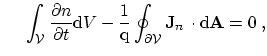
In general, the problem as defined in section Section 2.1.3 cannot be solved analytically. Thus, the solution has to be calculated by numerical methods, which normally require a discretization of the partial differential equations. For that reason, the domain $\mathcal{V}$ where the equations are posed has to be partitioned into a finite number of subdomains $\mathcal{V}_i$, which are usually obtained by a Voronoi tessellation [156,33]. In order to obtain the solution with a desired accuracy, the equation system is approximated in each of these subdomains by algebraic equations. The unknowns of this system are approximations of the continuous solutions at the discrete grid points in the domain [193].

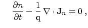
Several approaches for the discretization of the partial differential equations have been proposed. Due to the discretization of the current continuity equations it has been found to be advantageous to apply the finite boxes discretization scheme for semiconductor device simulation [193]. This method considers the equation integral form for each subdomain, which is the so-called control volume $\mathcal{V}_i$ associated with the grid point $\mathrm{P}_i$.

Before the Gauss integral theorem can be applied, the fluxes (2.58)-(2.60) are inserted in the balance equations (2.61)-(2.63) (analogously to the drift-diffusion model above):

$$\phantom{C_1} \displaystyle \frac{\displaystyle \partial n}{\disp... ...ensuremath{\ensuremath{\mathbf{\nabla}}}\cdot \ensuremath{\mathbf{J}}_n = 0 \ ,$$ (2.76)

$$C_1 \displaystyle \frac{\displaystyle \partial n T}{\displaystyle... ...nsuremath{\mathbf{J}}_n + n \, C_1 \, \frac{T - T_{\mathrm{L}}}{\tau_1} = 0 \ ,$$ (2.77)

$$C_2 \displaystyle \frac{\displaystyle \partial n T^2 \beta}{\disp... ...\mathbf{S}}_n + n \, C_2 \, \frac{T^2 \beta - T_{\mathrm{L}}^2}{\tau_2} = 0 \ .$$ (2.78)

The inner products $\ensuremath{\mathbf{F}}\cdot \ensuremath{\mathbf{J}}_n$ and $\ensuremath{\mathbf{F}}\cdot \ensuremath{\mathbf{S}}_n$ are discretized as [85]

$${ \ensuremath{\mathbf{F}}\cdot \ensuremath{\mathbf{J}}_n \,\Bigl\... ...nabla}}}\cdot \Bigl((\psi - \psi_i) \cdot \ensuremath{\mathbf{J}}_n \Bigr)\ , }$$ (2.79)

which can be handled in a straightforward way by employing the box integration method [193]. Consequently, equations (2.76)-(2.78) as well as the Poisson equation (2.21) are integrated resulting in

$${ \varepsilon \oint_{\partial \mathcal{V}}{\ensuremath{\ensuremat... ...\cdot \mathrm{d}{\mathbf{A}}} + \int_{\mathcal{V}}{\rho \, \mathrm{d}V} = 0 \ ,$$ (2.80)

$$\phantom{C_1} \int_{\mathcal{V}}{\displaystyle \frac{\displaystyl... ...l \mathcal{V}}{\ensuremath{\mathbf{J}}_n\,\cdot \mathrm{d}{\mathbf{A}}} = 0 \ ,$$ (2.81)

$$C_1 \int_{\mathcal{V}}{\displaystyle \frac{\displaystyle \partial... ...1 \, \int_{\mathcal{V}}{n \frac{T - T_{\mathrm{L}}}{\tau_1}\mathrm{d}V} = 0 \ ,$$ (2.82)

$$C_2 \int_{\mathcal{V}}{\displaystyle \frac{\displaystyle \partial... ...mathcal{V}}{n \frac{T^2 \beta - T_{\mathrm{L}}^2}{\tau_2}\mathrm{d}V} = 0 \ . {$$ (2.83)

Finally, the discretized equations are written implicitly as control functions:

$${ F_{\psi,i} = \varepsilon \sum_{j}{\frac{\psi_j - \psi_i}{d_{ij}} A_{ij}} + \rho_i V_i = 0 \ ,$$ (2.84)

$$F_{n,i} = \displaystyle \frac{\displaystyle \partial n}{\displaystyle \partial t} V_i - \frac{1}{\mathrm{q}} \sum_{j}{J_{n,ij} A_{ij}} = 0 \ ,$$ (2.85)

$$F_{T,i} = C_1 \displaystyle \frac{\displaystyle \partial n T}{\di... ...i) J_{n,ij} A_{ij}} + n \, C_1 \, \frac{T - T_{\mathrm{L}}}{\tau_1} V_i = 0 \ ,$$ (2.86)

$$F_{\beta,i} = C_2 \displaystyle \frac{\displaystyle \partial n T^... ...A_{ij}} + n \, C_2 \, \frac{T^2 \beta - T_{\mathrm{L}}^2}{\tau_2} V_i = 0 \ , {$$ (2.87)

with $d_{ij}$ as the distance between grid point $\mathrm{P}_i$ and $\mathrm{P}_j$, $A_{ij}$ as the interface area between the respective domains, and $V_i$ as the volumn of the domain. $J_{n,ij}$, $S_{n,ij}$, and $K_{n,ij}$ are the projections of the fluxes $\ensuremath{\mathbf{J}}_n$, $\ensuremath{\mathbf{S}}_n$, and $\ensuremath{\mathbf{K}}_n$ onto the edge $\ensuremath{\mathbf{e}}_{ij}$, respectively, and are evaluated at the center point of this edge. For the grid point $\mathrm{P}_i$ a general control function for the quantity $x$ is implicitly given as

$$F^\mathrm{S}_{x_{i}} = \sum_{j} F_{x_{ij}} + G_i = 0 \ ,$$ (2.88)

where $j$ runs over all neighboring grid points in the same segment, $F_{x_{ij}}$ is the flux between points $i$ and $j$, and $G_i$ is the source term (see Figure 2.1).

Figure 2.1: Box $i$ with six neighbors

Grid points on the boundary $\partial \mathcal{V}$ are defined as having neighbor grid points in other segments. Thus, (2.88) does not represent the complete control function $F_{x_i}$, since all contributions of fluxes into the contact or the other segment are missing. For that reason, the information for these boxes has to be completed by taking the boundary conditions into account. Common boundary conditions are the Dirichlet condition, which specifies the solution on the boundary $\partial \mathcal{V}$, the Neumann condition, which specifies the normal derivative, and the linear combination of these conditions giving an intermediate type:

$${ \ensuremath{\mathbf{n}} \cdot \ensuremath{\ensuremath{\ensuremath{\mathbf{\nabla}}}\, x} + \sigma x = \delta \ .}$$ (2.89)

Generally, the form of these conditions depends on the respective boundary models, and the conditions depend in turn on the interior information. For that reason, the equation assembly is often performed in a coupled way, causing complicated modules. For instance, it is absolutely necessary to differentiate between interior and boundary points. Considering a general tetrahedron, there exist many kinds of boundary points (depending on the number of edges involved), which have to be treated separately. This leads to a complicated implementation of the models and can make simplifications necessary. Thus, due to organizational and implementational issues this form of coupling should be avoided.

More complex models with exponential interdependence between the solution variables such as thermionic field emission interface conditions [185,201] have also been implemented.

A method has been under development to implement segment models calculating the interior fluxes and their derivatives independently from the boundary models. The segment models do not have to differentiate the point type, they do not even have to care about the boundary model used. The assembly system is responsible for combining all relevant contributions by using the information given by the boundary models.

2.2.1 Interface Conditions

To account for complex interface conditions, grid points located at the boundary of the segments (see Figure 2.2a) have three values, one for each segment (see Figure 2.2b) and a third point located directly at the interface which can be used to formulate more complicated interface conditions like for example, interface charges. However, to simplify notation these interface values will be omitted in the discussion and only the two interface points, $i$ and $i'$, are used.

Figure 2.2: Splitting of interface points: Interface points as given in a) are split into three different points having the same geometrical coordinates b)

Basically, the two (incomplete) equations $F^\mathrm{S}_{x_{i}}$ and $F^\mathrm{S}_{x_{i'}}$ are completed by adding the missing boundary fluxes $F_{x_{i,i'}}$:

$$F_{x_{i}} =~F^\mathrm{S}_{x_{i}} + F_{x_{i,i'}}~= 0 \ ,$$ (2.90)

$$F_{x_{i'}} =~F^\mathrm{S}_{x_{i'}} - F_{x_{i,i'}}~= 0 \ .$$ (2.91)

The intermediate type of interfaces (2.89) and thus also the two other types of interfaces are generally given in linearized form by:

$$\alpha(x_{i} - \beta x_{i'} + \gamma) = F_{x_{i,i'}} \ .$$ (2.92)

$\alpha$, $\beta$, and $\gamma$ are linearized coefficients, $F_{x_{i,i'}}$ represents the flux over the interface. The three types of interfaces differ in the magnitude of $\alpha$.

In the case of an arbitrary splitting of a homogenous region into different segments, the boundary models have to ensure that the simulation results remain unchanged. By adding (2.91) to (2.90), the box of grid point $\mathrm{P}_i$ can be completed and the boundary flux is eliminated. The merged box is now valid for both grid points, for that reason the respective equation cannot only be used for grid point $\mathrm{P}_i$, but also for $\mathrm{P}_{i'}$.

Whereas the segment models assemble the so-called segment matrix, the interface models are responsible for assembling and configuring the interface system consisting of a boundary and special-purpose transformation matrix. New equations based on (2.92) can be introduced into the boundary matrix without any limitations on $\alpha$, thus from 0 (Neumann) to $\infty$ (Dirichlet). The interface models are also responsible for configuring the transformation matrix to combine the segment and boundary matrix correctly. Depending on the interface type there are two possibilities:

• Dirichlet boundaries are characterized by $\alpha \rightarrow \infty$. Thus, the implicit equation $x_i = \beta x_{i'} - \gamma$ can be used as substitute equation. As these equations are normally not diagonally dominant they have a negative impact on the condition number and are configured to be preeliminated (see Section 4.8).
• For the other types (explicit boundary conditions) the boundary flux is simply added to the segment fluxes. In the case of a large $\alpha$, the transformation matrix could be used to scale the entries by $1/\alpha$ because of the preconditioner used in the solver module (see Section 4.10).

Note, that all interface-dependent information is administrated by the respective interface model only.

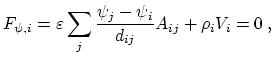
As an additional feature, the transformation matrix can be used to calculate several independent boundary quantities by combining the specific boundary value with the segment entries (also in the case of Dirichlet boundaries). For example, the dielectric flux over the interface is calculated as $\sum_i F^\mathrm{S}_{x_{i}}$ and introduced as a solution variable because some interface models require the cross-interface electric field strength to model effects such as tunnel processes. Calculation of the normal electric field is thus trivial. Note that this is not the case when the normal component of the electric field $\ensuremath{\mathbf{E}}_n$ has to be calculated using neighboring points when unstructured two- or three-dimensional grids are used.

See Figure 2.3 for an illustration of these concepts. The transformations are set up to combine the various segment contributions with the boundary system.

Figure 2.3: The complete equations are a combination of the boundary and the segment system. This combination is controlled by the transformation matrix and depends on the interface type. In the upper figure, the case for Dirichlet boundary conditions including substitute equations is shown, in the lower figure for all other cases.

2.2.2 Boundary Conditions

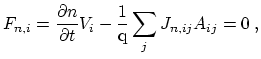
Contacts are handled in a similar way to interfaces. However, in the contact segment there is only one variable available for each solution quantity ( $x_{\mathrm{C}}$). Note that contacts are represented by spatial multi-dimensional segments. Furthermore, all fluxes over the boundary are handled as additional solution variables $F_{\mathrm{C}}$ (for example, contact charge $Q_{\mathrm{C}}$ for the Poisson equation, contact electron current $I_{n_{\mathrm{C}}}$ for the electron continuity equations, or $H_\mathrm{C}$ as the contact heat flow).

For explicit boundary conditions one gets

$${ F_{x_{i}} =F^\mathrm{S}_{x_{i}} + F_{x_{i,{\mathrm{C}}}} = 0 \ ,$$ (2.93)

$$F_{F_{\mathrm{C}}} =F_{\mathrm{C}} + \sum_i F^\mathrm{S}_{x_{i}} = 0 \ ,{$$ (2.94)

with $i$ running over all segment grid points.

At Schottky contacts explicit boundary conditions apply. The semiconductor contact potential $\psi_{\mathrm{s}}$ is fixed and given as the difference of the metal quasi-Fermi level (which is specified by the contact voltage $\psi_{\mathrm{C}}$) and the metal workfunction difference potential $\psi_{\mathrm{wf}}$.

$$\psi_{\mathrm{s}}= \psi_{\mathrm{C}}-\psi_{\mathrm{wf}},\hspace{5... ...{where}}\hspace{5mm} \psi_{\mathrm{wf}}= -\frac{E_{\mathrm{w}}}{\mathrm{q}} \ .$$ (2.95)

The difference between the conduction band energy $E_{\mathrm{C}}$ and the metal workfunction energy gives the workfunction difference energy $E_{\mathrm{w}}$ which is the barrier height of the Schottky contact.

For Dirichlet boundary conditions one gets

$${ F_{x_{i}} =x_{\mathrm{C}} - h(x_{i}) = 0 \ ,$$ (2.96)

$$F_{F_{\mathrm{C}}} =F_{\mathrm{C}} + \sum_i F^\mathrm{S}_{x_{i}} = 0 \ .{$$ (2.97)

Here, $x_{\mathrm{C}}$ is the boundary value of the quantity, which is a solution variable, whereas (2.97) is used as constitutive relation for the actual flow over the boundary $F_{\mathrm{C}}$.

For example, at Ohmic contacts simple Dirichlet boundary conditions apply. The contact potential $\psi_{\mathrm{s}}$, the carrier contact concentrations $n_s$ and $p_s$, and in the energy-transport simulation case, the contact carrier temperatures $T_n$ and $T_p$ are fixed. The metal quasi-Fermi level (which is specified by the contact voltage $\psi_{\mathrm{C}}$) is equal to the semiconductor quasi-Fermi level. With the constant built-in potential $\psi_{\mathrm{bi}}$ (calculated after [65]), the contact potential at the semiconductor boundary reads

$$\psi_{\mathrm{s}}= \psi_{\mathrm{C}}+ \psi_{\mathrm{bi}}.$$ (2.98)

For Neumann boundaries the flux over the boundary is zero hence the equation assembled by the segment model is already complete.