Subsections

• 4.7.1 Row Transformation
• 4.7.2 Variable Transformation

4.7 Compiling the Complete Linear Equation System

After the assembly process has been finished, all four matrices and two vectors have to be compiled to obtain the complete linear equation system. The first step is to compile the segment and the boundary system in the following way:

$$\ensuremath{\mathbf{b}} = {\ensuremath{\ensuremath{\mathbf{b}}_{\... ...athbf{T}}_{\mathrm{b}}}} {\ensuremath{\ensuremath{\mathbf{b}}_{\mathrm{s}}}}\ ,$$ (4.9)

$$\ensuremath{\mathbf{A}} = {\ensuremath{\ensuremath{\mathbf{A}}_{\... ...athbf{T}}_{\mathrm{b}}}} {\ensuremath{\ensuremath{\mathbf{A}}_{\mathrm{s}}}}\ ,$$ (4.10)

$$\ensuremath{\mathbf{A}} \ensuremath{\mathbf{x}} = \ensuremath{\mathbf{b}}\ ,$$ (4.11)

$$({\ensuremath{\ensuremath{\mathbf{A}}_{\mathrm{b}}}} + {\ensurema... ...athbf{T}}_{\mathrm{b}}}} {\ensuremath{\ensuremath{\mathbf{b}}_{\mathrm{s}}}}\ .$$ (4.12)

The second compilation step regards the variable transformation matrix $\ensuremath{\mathbf{T}}_{\mathrm{v}}$:

$$(({\ensuremath{\ensuremath{\mathbf{A}}_{\mathrm{b}}}} + {\ensurem... ...thbf{T}}_{\mathrm{b}}}} {\ensuremath{\ensuremath{\mathbf{b}}_{\mathrm{s}}}})\ .$$ (4.13)

The left side of Figure 4.2 shows the completely compiled system matrix arising from the discretization of a two-dimensional MOS transistor structure. Since the linear equation systems has been assembled by the drift-diffusion models of MINIMOS-NT, it consists of three major quantities. For the semiconductor segment, the values of and the couplings between the potential (row or column number 45-955), electron (956-1879) and hole concentrations (1880-2803) can be clearly seen. After the discussions of the pre-elimination, the sorting, and the scaling, the respective graphical representations of the same system matrix will be shown.

In the next sections the row and variable transformations are going to be discussed in a more detailed way.

4.7.1 Row Transformation

As already discussed in Section 4.6, semiconductor device simulation based on the finite volume method is used as an example to discuss the row transformation. The complete linear equation system is built from a segment system, which is the segment system matrix $\ensuremath{\mathbf{A}}_{\mathrm{s}}$ and the segment right-hand-side vector $\ensuremath{\mathbf{b}}_{\mathrm{s}}$, both of them representing cumulated fluxes and their derivatives to the system variables. Basically, the fluxes are calculated from segment models describing the interior of discretized regions. The matrix is a linear superposition of very small matrices, one for each flux, with few non-zero elements only. Consequently, the same superposition applies for the vector $\ensuremath{\mathbf{b}}_{\mathrm{s}}$.

All fluxes are assigned to boxes, a box is in turn assigned to each variable. As the control function for a box is defined by the user, for example being the sum of all fluxes leaving the box, the fluxes leaving the boxes are entered into the vector $\ensuremath{\mathbf{b}}_{\mathrm{s}}$ in the places appropriate for the variables that are assigned to the boxes. In context of the Newton method, $\ensuremath{\mathbf{A}}_{\mathrm{s}}$ is part of the Jacobian matrix and contains the negative derivatives of the values in $\ensuremath{\mathbf{b}}_{\mathrm{s}}$ to the system variables. The right-hand-side vector depends on the current solution of the Newton iteration.

The boundary conditions will enforce some special physical conditions at the boundaries. The control functions of boxes along the boundaries will usually be completed by the boundary conditions. For example, a Dirichlet boundary condition will use the dielectric flux cumulated in the boundary box to calculate the surface charge on the surface of the adjacent material. The equation used to calculate the value of the boundary variable, however, will not always make use of the fluxes accumulated in the segment system.

The boundary conditions are therefore implemented by two elements: a boundary system ( $\ensuremath{\mathbf{A}}_{\mathrm{b}}$ and $\ensuremath{\mathbf{b}}_{\mathrm{b}}$) and a transformation matrix $\ensuremath{\mathbf{T}}_{\mathrm{b}}$. The purpose of the matrix $\ensuremath{\mathbf{T}}_{\mathrm{b}}$ is the forwarding of the fluxes of the main system to their final destinations or their resetting if they are not required. The system of $\ensuremath{\mathbf{A}}_{\mathrm{b}}$ and $\ensuremath{\mathbf{b}}_{\mathrm{b}}$ represents additional or, in case of Dirichlet boundary conditions, substitutional parts of the final equation for the variables at the boundaries. Again, the entries in the matrix $\ensuremath{\mathbf{A}}_{\mathrm{s}}$ are the negative derivatives of the right-hand-side vector $\ensuremath{\mathbf{b}}_{\mathrm{b}}$ to the variable vector $\mathbf{v}$.

4.7.2 Variable Transformation

Especially in the case of mixed quantities in the solution vector, a variable transformation is sometimes helpful to improve the condition of the linear system. The representation chosen here allows to specify fairly arbitrary variable transformations to be applied to the system. Basically, a matrix $\ensuremath{\mathbf{T}}_{\mathrm{v}}$ is assembled and multiplied with the system matrix from the right.

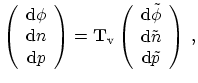
For example, to reduce the coupling of the semiconductor equations and thus improve the condition of the system matrix, a transformation of the stationary drift-diffusion model is suggested in [10]. The system matrix can be diagonalized to leading terms by substituting $\ensuremath{\mathrm{d}\phi}$, $\ensuremath{\mathrm{d}n}$, and $\ensuremath{\mathrm{d}p}$ by

$$\left( \begin{array}{c} \ensuremath{\mathrm{d}\phi}\\ \ensuremath... ...{\mathrm{d}\tilde{n}}\\ \ensuremath{\mathrm{d}\tilde{p}} \end{array} \right)\ ,$$ (4.14)

$$\ensuremath{\mathbf{\tilde{A}}} = \ensuremath{\mathbf{A}} {\ensuremath{\ensuremath{\mathbf{T}}_{\mathrm{v}}}}\ ,$$ (4.15)

$$\ensuremath{\ensuremath{\mathbf{T}}_{\mathrm{v}}}= \left( \begin{... ...hrm{q}}{\ensuremath{\mathrm{k_B}}T_{\mathrm{L}}} & 0 & 1 \end{array} \right)\ .$$ (4.16)

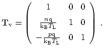
This transformation is the Gummel-Ascher transformation, and was extended for the differential equations of the energy-transport model in [201]:

$$\ensuremath{\ensuremath{\mathbf{T}}_{\mathrm{v}}}= \left( \begin{... ... & 0 \\ [2mm] 0 & 0 & \frac{\ensuremath{T_p}}{p} & 0 & 2 \end{array} \right)\ .$$ (4.17)

The Gummel-Ascher transformation meets all requirements for such variable transformations: first the transformation is expressed by a matrix ${\ensuremath{\ensuremath{\mathbf{T}}_{\mathrm{v}}}}$ which has an inverse ${\ensuremath{\ensuremath{\mathbf{T}}_{\mathrm{v}}^{-1}}}$. Second, it does not destroy the diagonal dominance. In fact there is no qualitative difference between $\ensuremath{\mathbf{A}}$ and $\ensuremath{\mathbf{\tilde{A}}}$ in terms of this condition property because the original system is substituted by a related one (see (4.14)). Third, the transformation matrix decomposes into small submatrices with a limited number of variables involved in a single transformation. The variable transformation is restricted to variables on the specific grid points, thus, it is a local transformation.

For compactness, the following substitutions will be used hereafter for the complete linear equation system:

$${\ensuremath{\tilde{\ensuremath{\mathbf{A}}}}} = (({\ensuremath{\... ...hbf{A}}_{\mathrm{s}}}}) {\ensuremath{\ensuremath{\mathbf{T}}_{\mathrm{v}}}})\ ,$$ (4.18)

$${\ensuremath{\tilde{\ensuremath{\mathbf{x}}}}} = ({\ensuremath{\ensuremath{\mathbf{T}}_{\mathrm{v}}^{-1}}} \ensuremath{\mathbf{x}})\ ,$$ (4.19)

$${\ensuremath{\tilde{\ensuremath{\mathbf{b}}}}} = ({\ensuremath{\e... ...thbf{T}}_{\mathrm{b}}}} {\ensuremath{\ensuremath{\mathbf{b}}_{\mathrm{s}}}})\ .$$ (4.20)