4.2.5 Solver
The discretization of a PDE results typically in an equation system  . Solving
a large system of equations is computational expensive and consequently direct
methods, like the Gaussian elimination procedure, cannot be applied in practice due
to inadmissible execution times. Therefore, iterative solving procedures, like the
conjugate-gradient [118] and the generalized minimal residual method [119] methods, are
usually applied.
. Solving
a large system of equations is computational expensive and consequently direct
methods, like the Gaussian elimination procedure, cannot be applied in practice due
to inadmissible execution times. Therefore, iterative solving procedures, like the
conjugate-gradient [118] and the generalized minimal residual method [119] methods, are
usually applied.
The convergence behavior of these approaches can be further improved by
preconditioners [120], such as the Jacobi method and the family of incomplete lower upper
factorization methods. It is obvious, that the nature of the assembled PDE, whether it is linear
or nonlinear, determines the solution procedure of the equation system. Non-linear systems
are commonly solved by Newton-type methods.
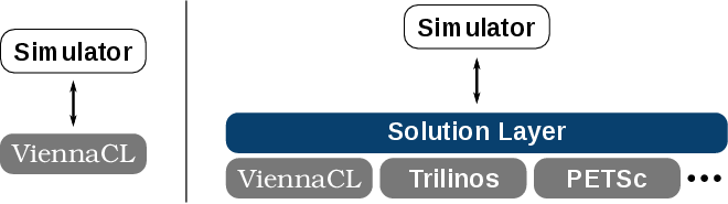
Several libraries are available which provide relevant tools for solving large systems of
equations [1][121][122]. Consequently, the different solver approaches and the different
libraries introduce a plethora of prerequisites by the respective API. In order to retain
utmost flexibility for a device simulator, the design has to deal with these inconsistent
solver interfaces by decoupling the solver backends from the actual implementation
(Figure 4.8).