Subsections

• 2.2.1 Vertex Insertion Methods
• 2.2.2 Tetrahedral Bisection
• 2.2.3 Recursive Tetrahedral Bisection
  • 2.2.3.1 A Recipe

2.2 Tetrahedral Partitioning Methods

Mesh adaptation procedures in general can be grouped into three different methods, depending on the level of mesh modifications. As discussed in [34] these groups are named r-, p-, and h-methods. Where in the following r- and p-methods are just discussed briefly, h-techniques for tetrahedral meshes are examined in detail.

Using the r-method, the mesh connectivity is unchanged. Instead, node relocation is used to move the mesh nodes, either by means of weighted barycentric smoothing based on the location and the weight of the nodes in some neighborhood, or by means of element distortion. The criteria (weights) governing these operations are obtained by analyzing the local mesh quality not only in a geometric sense, also rules for different discretization schemes can be used. For this method the mesh modification level is normally low, so the r-method is used as a ``mesh fine tuning'' method.

The p-method approach is based on an invariant mesh (in terms of points (nodes, vertexes) and elements) and adjusts the degree (in terms of the interpolation functions) of the used discretization scheme constructed on the mesh elements as a function of the current solution analysis. This method is very popular for finite element discretization where also mixed forms of p-, and h-methods are in use. An overview of basic principles and properties for p- and for hp-methods is given in [35]. Introductory concepts for linear and second order approximation schemes, which are subsets of general polynomial approximations are discussed in Section 3.1.3.

Adaptation by the h-method is defined in terms of local or global mesh enrichment by means of refining (by partitioning) or coarsening selected elements or all elements in a mesh.

The following deals mostly with three-dimensional simplex partitioning based on the so-called tetrahedral bisection method. In addition, an overview is given of a more general class of adaptation processes, the so-called vertex insertion methods. Higher h-adaptation methods like the red-green refinement methods or the $n$ -dimensional extension of the $4T$ algorithm can be found in literature [36,37,38], but these methods are not subject of further discussions.

2.2.1 Vertex Insertion Methods

To achieve local three-dimensional simplex partitioning three configurations of inserting a new vertex (node) are possible [4]. It is likely to define a new vertex along an edge, on a face, or inside a tetrahedron as depicted in Figure 2.1.

Figure 2.1: Local three-dimensional simplex partitioning. One new vertex can be inserted on an edge, a face, or in the interior of an initial tetrahedron. The original tetrahedron is then cut into two, three, or four tetrahedrons, respectively.

Depending on the location of the new vertex, the initial tetrahedron is split into two, three, or four tetrahedra respectively, where the last case (see Figure 2.1(d) and Figure 2.1(h)) does not influence neighboring tetrahedra at all. For a new vertex located on a face (see Figure 2.1(c) and Figure 2.1(g)) the spatial influence of the portioning process is limited to the face neighbor of the initial tetrahedron which is also split into three pieces just in a mirrored way. For the first case (see Figure 2.1(b) and Figure 2.1(f)), where a new vertex is located on an edge of an initial tetrahedron the influence can not be simple predicted since the whole edge batch, i.e. all tetrahedra which share the edge of the new vertex, are influenced and split into two pieces. This local partitioning method is therefore called tetrahedral bisection which is subject of Section 2.2.2.

2.2.2 Tetrahedral Bisection

Tetrahedral bisection is a special kind of h-method adaptation where only mesh refinement by inserting a vertex on an edge, the so-called refinement edge, is allowed [39]. According to Figure 2.1, this is the most left case (Figure 2.1(b) and Figure2.1(f)), where the original tetrahedron is split into two new ones, the algorithm is therefore called tetrahedral bisection. In the literature, one can find different improvements and specifications for this algorithm, e.g. in [40], however, one common problem is how to detect a particular edge, the refinement edge, as supporter for the new vertex. In a mesh, tetrahedrons are not isolated and inserting a new vertex influences the whole edge batch of the refinement edge, if the conformity of the mesh after the refinement step should be kept, which is normally the case. Figure 2.2 shows a constellation of four tetrahedrons. For the refinement edge, the bold red line in the middle was chosen. After insertion of the new vertex the refined constellation carries, in this example case, eight tetrahedra.

Figure 2.2: Inserting a new vertex on a particular edge - the so-called refinement edge - yields to bisection of all tetrahedra which are connected to the refinement edge. This h-refinement-method (see Section 2.2) is therefore called tetrahedral bisection.

The selection process of a particular refinement edge influences the element shape of the refined constellation in a very strong way. Different element shape measures are used for the evaluation of the element quality [41] after tetrahedral bisection not only in a geometric way, also based on demands of different discretization schemes and applications. For instance in Section 4, the bisection algorithm is controlled by the simulation of a diffusion process whereby the accuracy of the simulation is improved through mesh refinement.

One very common variant of the bisection algorithm is the so-called longest edge bisection method [42]. The basic idea is to choose the longest edge of a triangle or tetrahedron as refinement edge to optimize the shape of the refinement element. In general, elements become more isotropic and therefore, obtuse face angles can be avoided, which has a positive impact to a discretization scheme of finite elements [43]. One has to keep in mind that for general constellations the refinement edge is not necessary the longest edge of all involved mesh elements. Such configurations can be treated in a special way or ignored if higher geometric element distortions are welcome.

One method to handle configurations where the refinement edge is not the longest edge of all involved tetrahedra is the so-called recursive tetrahedral bisection approach. This method can be used to avoid higher distorted elements, on the other hand, this characteristic is paid with a violation of the refinement locality, i.e. in a recursive tetrahedral bisection algorithm the locality of the refinement procedure is no longer guaranteed. A second counterbalance is that special care has to be taken on the termination of the algorithm since endless recursion is possible. The basic concepts of this method are subject of the following section, an extension of this algorithm for volitional geometrically distorted elements is presented in Section 2.3.2.

2.2.3 Recursive Tetrahedral Bisection

For further investigations it is useful to introduce a new term for tetrahedral meshes, which defines an exceptional relation between neighboring tetrahedra [44].

Definition 11 (Compatibly divisible)   A $3$ -simplex is said to be compatibly divisible if and only if its refinement edge (see Section 2.2.2) is either the refinement edge of all other $3$ -simplices sharing the refinement edge or the edge is part of the boundary of the domain.

Remark 2 (Refinement edge)   In Definition 11 the process of specifying a particular refinement edge of a tetrahedron is not defined at all. So this parameter can be freely chosen but should be always deterministic.

In Section 2.2.2 (see Figure 2.2) a constellation is shown, where the Euclidian length was chosen for the specification of the refinement edge, i.e. that the longest edge of each tetrahedra is marked as refinement edge. In this particular case the refinement edges of all tetrahedra are identical, so Definition 11 holds and therefore the batch is said to be  compatibly divisible. More challenging is the case of non-compatibly divisible tetrahedra batches and the transformation into compatibly divisible configurations via recursive tetrahedral bisection which is part of the following.

Figure 2.3: Figure 2.3(a) and Figure 2.3(c) jointly show two tetrahedra with different refinement edges, colored red and blue. The constellation is said to be non-compatibly divisible because refinement edges of neighboring tetrahedra are not identical. Figure 2.3(b) and Figure 2.3(d) show the resulting configuration where the red refinement edge was chosen for the bisection.

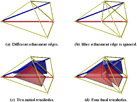Figure 2.3(c) shows two tetrahedra colored red and blue in a neighboring relation, where the corresponding edge representation is given in Figure 2.3(a). For the refinement edge of each tetrahedron simple the edge with the longest Euclidian length was chosen and colored according the colors of the belonging tetrahedra. So one can see that the constellation depicted in Figure 2.3 does not fulfill Definition 11 because the red and the blue refinement edges are not identical and therefore this configuration is non-compatibly divisible.

Using tetrahedral bisection (see Section 2.2.2) and starting randomly with the red tetrahedra and ignoring the neighboring constellation (blue tetrahedron) yields to four tetrahedra depicted in Figure 2.3(b) and Figure 2.3(d) jointly. Focused on the new two blue tetrahedra, it is clear that the left one is more prolated than the nearly regular initial blue one. This kind of distortion is characteristic for tetrahedral bisection.

Figure 2.4: Compared to Figure 2.3 in this case the blue refinement edge is not ignored and chosen for the first refinement step. This additional step solves the non-compatibly divisible problem and the red refinement edge can be bisected afterwards. This recursive process yields more regular mesh elements compared to obstinate tetrahedral bisection.

Figure 2.4 shows the evolution of the so-called recursive tetrahedral bisection approach. Once again we start in the same constellation as shown in Figure 2.3, with two tetrahedra in a non-compatibly divisible configuration and the red tetrahedron is randomly chosen for the first refinement step. A compatibly divisible test shows, that the neighboring blue tetrahedron does not fulfill Definition 11 and so we chose the violating tetrahedra (the blue one) as first refinement tetrahedra. For the blue tetrahedron Definition 11 holds, because the refinement edge is part of the boundary of the domain and can therefore be used for a tetrahedral bisection step. The result of this process is shown in Figure 2.4(b) and Figure 2.4(e) jointly. Now there is only one refinement edge left (the red one) where once again a compatibly divisible test is carried out. Now the test allows to use the red refinement edge, because all influenced tetrahedra fulfill Definition 11. The final result is shown in Figure 2.4(c) and Figure 2.4(f), respectively, which holds five tetrahedra, three blue and two red ones. The three blue ones become more regular than the two blue ones produced by obstinate tetrahedral bisection as shown in Figure 2.3. It is in the nature of this algorithm to avoid highly prolated elements if the Euclidian length is used for the specification of the refinement edge.

For more general configurations where more than two tetrahedra are involved, the refinement mechanism for violating tetrahedra (blue one first) can be repeated as long as they exist. This repetition can be expressed through a recursive definition which yields the term recursive tetrahedral bisection [45].

2.2.3.1 A Recipe

The choice of the longest edge as refinement edge criterion used during recursive tetrahedral bisection appears to be good from a geometrical point of view, since the upcoming mesh elements become more regular. On the other hand side, the depth of the recursion can become very deep, especially in the case of poor regular mesh elements, where no unique longest edge can be detected, and the refinement edge must be chosen randomly. Also the worst case, endless recursion cannot be detected a priori and deterministicly avoided. This notice yields a limitation of the recursion depth to an adjustable limit.

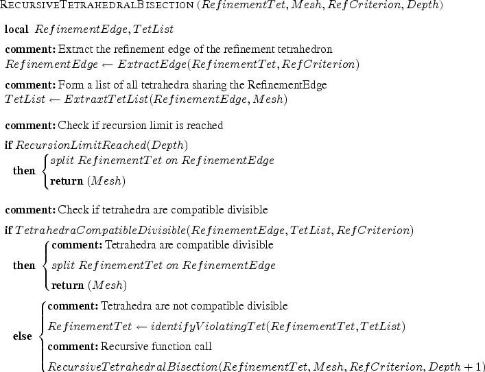
Table 2.1 gives a pseudo-code fragment which shows the nature of the recursive tetrahedral bisection algorithm where the limitation of the recursion depth also has been taken under consideration.

Table 2.1: Algorithm; Recursive tetrahedral bisection.

In Section 2.3.2 the influence of a non-constant metric for the calculation of an edge's length is investigated, which broadens the abilities of recursive tetrahedral bisection dramatically. But first a closer look on defining a metric and incorporate the capacity of anisotropy is necessary.