


Next: 5.2.2 Interface Transport
Up: 5.2 Charge Transport in
Previous: 5.2 Charge Transport in
In the bulk only the ions are engaged in the charge transport. The charge transfer behaves similar to that in a resistor. Thus, it is adequate to find an accurate formulation for the resistivity of the bulk electrolyte in order to fully characterize transport. Often, the conductivity of electrolytes is expressed via their molar conductivity. Determing the molar conductivity is a delicate task, due to the many parameters influencing it. The ionic concentration and the valence in the solution play important roles in determing the conductivity of the bulk electrolyte. Furthermore, the degree of ionic dissociation also influences the total resistivity of the solution. For instance,
 of acetic acid
 and
and  exhibit different conductivities. Even though both solutions posses univalent bonds, their dissociation constants are different.
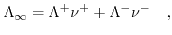
has a much smaller dissociation constant and, therefore, the number of ions is much smaller than that for the solution. Increasing the ion concentration of the solution raises the number of charge carriers. Increasing the number of charge carries also means increasing the electrostatic interaction between the ions and thus decreasing the mobility. Kohlrausch's law covers this behavior for strong (fully dissolved) and dilute electrolytes[191]:
exhibit different conductivities. Even though both solutions posses univalent bonds, their dissociation constants are different.
has a much smaller dissociation constant and, therefore, the number of ions is much smaller than that for the solution. Increasing the ion concentration of the solution raises the number of charge carriers. Increasing the number of charge carries also means increasing the electrostatic interaction between the ions and thus decreasing the mobility. Kohlrausch's law covers this behavior for strong (fully dissolved) and dilute electrolytes[191]:
 |
(5.7) |
where
 denotes the molar conductivity of an electrolyte at infinite dilution.
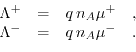
 and
and
 are the molar conductivities for positive and negative ions, and
  and
and  describe the valences of the corresponding ions. (5.7) presumes neglible ionic interactions between counterions for strong, dilute electrolytes and that the overall conductivity can be calculated via the sum of the positive and the negative molar conductivity weighted with their corresponding ion valence. The molar ionic conductivity is connected with the ionic mobility through:
 |
(5.8) |
Here,  denotes the elementary charge,
  Avogrado's constant and
  the ionic mobility for positive/negative ions. The molar conductivity at infinite dilution
preumes that ionic interactions have not yet started to impede the conductivity of the solution due to the infinite distance between the ions.
The following law allows an estimation of the relation between the effective conductivity
the ionic mobility for positive/negative ions. The molar conductivity at infinite dilution
preumes that ionic interactions have not yet started to impede the conductivity of the solution due to the infinite distance between the ions.
The following law allows an estimation of the relation between the effective conductivity  and the molar concentration
 ![$ [c]$](img727.png) 5.1:
5.1:
![$\displaystyle \Lambda=\Lambda_{\infty} - K \sqrt{\left[c\right]}\quad.$](img728.png) |
(5.9) |
Since, similar forces affect the ions as those affecting electrons in metal resistors, the motion of the ions can be modeled by a resistor [191]. The value of the resistor can be deduced from (5.7)-(5.9) under the assumption of known concentrations and mobilities for the contributing ionic components.
Footnotes
- ...5.1
 denotes the Kohlrausch coefficient.
Next: 5.2.2 Interface Transport
Up: 5.2 Charge Transport in
Previous: 5.2 Charge Transport in
T. Windbacher: Engineering Gate Stacks for Field-Effect Transistors