6.3 Analytical Comparison between the Poisson-Boltzmann, the Extended Poisson-Boltzmann, and the Debye-Hückel Model

For better comparison between the Poisson-Boltzmann, the extended Poisson-Boltzmann, and the Debye-Hückel model we study their one-dimensional analytical solutions without any charges from macromolecules or due to the site-binding effect at the oxide surface. The surface potential $\varphi_{0}$ will be chosen in a way that all models exhibit the same charge at the surface and that the potential $\varphi$ and the electric field $\mathcal{E}$ vanish in the limit of infinite distance away from the surface. In the first step all equations are transformed to dimensionless units.

Reformulating the Laplace term

$$\frac{d\varphi^{2}}{dz^{2}} = -\frac{d\mathcal{E}}{dz} = \mathcal{E}\cdot \frac{d\mathcal{E}}{d\varphi}$$ (6.14)

and transforming the equations with

$$\begin{array}{ccc} \varphi &=& \frac{q \psi}{k_{\text{B}} T}\... ...T\varepsilon_{0} \varepsilon_{\mathrm{sol}}}\quad , \end{array}$$ (6.15)

leads to the following differential equations:

$$\mathcal{E}\cdot \frac{d\mathcal{E}}{d\varphi} = \frac{1}{\lambda_{\mathrm{D}}^{2}}\, \sinh \left( \varphi \right)$$ (6.16)

for the Poisson-Boltzmann model,

$$\mathcal{E}\cdot \frac{d\mathcal{E}}{d\varphi}=\frac{2}{\lambda_{... ...phi/2) )\sinh ( \varphi/2 )}{\left( (1-a) + a \cosh(\varphi/2)\right)^{3}}\quad$$ (6.17)

for the extended Poisson-Boltzmann model and

$$\mathcal{E}\cdot \frac{d\mathcal{E}}{d\varphi} = \frac{1}{\lambda_{\mathrm{D}}^{2}}\, \varphi \quad,$$ (6.18)

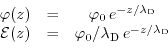
for the Debye-Hückel model.

Assuming vanishing potential $\varphi$ and vanishing electric field $\mathcal{E}$ for large distances $z\rightarrow\infty$, integrating these equations twice results in the following solutions:

$$\begin{array}{ccc} \varphi(z) & = &\displaystyle{2 \ln \left(... ...a_{\mathrm{D}}} \tanh^{2} (\varphi_{0}/4)}} \quad , \end{array}$$ (6.19)

for the Poisson-Boltzmann model [227],

$$\begin{array}{ccl} z(\varphi)& = &-\lambda_\mathrm{D}\,\ln\le... ...left(\frac{\varphi_{0}}{2}\right)}\right\vert\quad, \end{array}$$ (6.20)

or via $\mathcal{E}$ as a function of $\varphi$

$$\mathcal{E}(\varphi) = \frac{2}{\lambda_{\mathrm{D}}} \frac{\sinh(\varphi/2)}{1-a+a \cosh(\varphi/2)}\quad,$$ (6.21)

for the extended Poisson-Boltzmann model [225], and

$$\begin{array}{ccc} \varphi(z) & = & \varphi_{0}\, e^{-z/\lamb... ...\lambda_{\mathrm{D}}}\, e^{-z/\lambda_{\mathrm{D}}} \end{array}$$ (6.22)

for the Debye-Hückel model [226].

Unfortunately the analytical expression (6.27) is not as handy as the expressions (6.30) for the Debye-Hückel model and (6.25) for the Poisson-Boltzmann model. As can be seen in (6.27), only for the position $z$ as a function of the potential $\varphi$ it is possible to write down a compact analytical expression, while for the inverse function one has to use numerical approaches. However, in the limit $a\rightarrow 0$ the solution for the Poisson-Boltzmann model is recovered [225].

In the next step we assume an equivalent surface charge $\sigma _{0}$ for all three models, in order to accomplish a better comparison between them. This is realized by choosing an arbitrary charge at the surface and applying Gauß's law. This way, a surface potential $\varphi_{0}$ related to the same surface charge can be found.

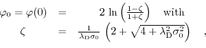
The corresponding surface potentials are:

$$\begin{array}{ccc} \varphi_{0}=\varphi(0)&=&2\,\ln \left(\fra... ...lambda_{\mathrm{D}}^{2}\sigma_{0}^{2}}\right)\quad, \end{array}$$ (6.23)

for the Poisson-Boltzmann model [227],

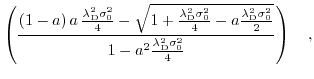$$\varphi_{0}=\varphi(0)=-2\, \left(\frac{\left(1-a\right) a\, \frac{\lambda_{\mathrm{D}}^{2} \... ...}{2}}}{1-a^{2} \frac{\lambda_{\mathrm{D}}^{2} \sigma_{0}^{2}}{4}}\right) \quad,$$ (6.24)

for the extended Poisson-Boltzmann model [225], and

$$\varphi_{0}=\varphi(0)=\lambda_{\mathrm{D}}\,\sigma_{0}\quad,$$ (6.25)

the Debye-Hückel model, respectively.

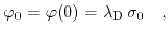
Figure 6.5: Illustrating the different screening characteristica for the Poisson-Boltzmann, the extended Poisson-Boltzmann, and the Debye-Hückel model. In the limit of $a\rightarrow 0$ the extended Poisson-Boltzmann model rejoins the Poisson-Boltzmann model, while for increasing closest possible ion distance $a$, which corresponds to a decreasing salt concentration, the screening is reduced and resembles for $a=0.275$ the Debye-Hückel model.

Fig. 6.5 shows a comparison between the Poisson-Boltzmann, the extended Poisson-Boltzmann, and the Debye-Hückel model. As already mentioned before, one can see that for $a\rightarrow 0$ the extended Poisson-Boltzmann model and the Poisson-Boltzmann model coincide. Increasing the closest possible approach $a$ between two ions, leads to a reduction in screening and thus higher surface potential $\varphi_{0}$. Furthermore, for $a=0.275$ the extended Poisson-Boltzmann model equations quite well with the Debye-Hückel model. This shows that the extended Poisson-Boltzmann model is able to cover a wider range of screening behavior than the Poisson-Boltzmann and the Debye-Hückel model.