


Next: 6.3 Analytical Comparison of
Up: 6.2 Modeling BioFETs
Previous: 6.2.5 Debye-Hückel Model
Subsections
Normally, the experiment is carried out in a so called buffer solution. There are several reasons for this. For instance, enzyme reactions are very sensitive to the local temperature, the local substrate concentration, and also to their chemical environment (e.g. pH). In this case the buffer fulfills the function of stabilizing the pH of the solution at a certain point and thus keeping the enzyme activity at its maximum. If DNA is going to be hybridized6.3, the ions in the buffer gather around the single DNA strands and screen partially the DNA charge. The repulsion between the two negatively charged single DNA strands is reduced and they can approach each other close enough to enable the hybridization reaction.
The utilization of buffers is a path way to control the chemical properties of the environment in which the chemical reaction is conducted. Therefore, buffers are also a significant ingredient in the description of BioFETs and a method to calculate the ion concentrations and the ionic strength for an arbitrary buffer will be given. Beynon and Easterby published a book about buffer solutions, giving an exhaustive and easy introduction into this topic [5].
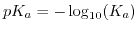 is, analogously to the definition of the pH of a solution, for the reaction
  . Since the equilibrium constant of a buffer is determined by the laws of thermodynamics, it has to depend on temperature. This is described by
 , the change of
  with temperature. The logarithmized equilibrium constant depends on the applied buffer and can exhibit positive or negative values, or even being close to zero. Therefore,
 |
(6.9) |
 denotes the temperature and represents the thermodynamic value for
 .
.
Biological sensors are typically employed at a certain pH. The pH can be adjusted by tritration and monitored by measurement. Hence, pH is an input parameter for the simulation. Starting with a given pH, the buffer ion concentrations can be calculated including temperature effects and the ionic strength of the solution.
 determines the buffer ion concentrations but also depends on the ionic strength
 and temperature . Since the ionic strength also depends on the buffer ion concentration, this nonlinear equation system has to be solved self-consistently. The effect of the ionic strength
on
and temperature . Since the ionic strength also depends on the buffer ion concentration, this nonlinear equation system has to be solved self-consistently. The effect of the ionic strength
on
 can be compressed in one relation (also known as the Debye-Hückel relationship):
![$\displaystyle pK^{\prime}_{a, T} = pK_{a, T} + \left(2\,\xi_{a}-1\right) \left[\frac{A\sqrt{I}}{1+\sqrt{I}}-0.1\, I \right]\quad.$](img859.png) |
(6.10) |
is termed as modified, working, or practical value,  is the charge on the conjugate acid species and
  is a temperature dependent constant.
  is normally around
  (at
(at
 and at
 ). Furthermore,
 is a function of position, because the ionic strength exhibits a position dependence, while
  is only related to temperature.
The Henderson-Hasselbach equation connects the relative concentrations of acid and base and the
of the conjugate acid/base pair to the pH of the electrolyte,
![$\displaystyle pH=pK^{\prime}_{a, T} + \log_{10}\left( \frac{\left[\mathrm{acid}\right]}{\left[\mathrm{base}\right]}\right)\quad.$](img867.png) |
(6.11) |
On account of the spatial coordinate dependence of all input quantities, the local pH is also a function of position. In the vicinity of the interface the pH value will deviate from the pH value in the bulk electrolyte. Remembering that the ion concentrations are also related to the local potential via the Poisson-Boltzmann equation, further complicates the situation. In order to include all effects one has to employ a numerical approach and solve the equations in a self-consistent manner.
A feasible algorithm works as follows:
- Define the temperature and the bulk pH value.
- Define a buffer. Normally there is already one specified from an experiment. If none is available, choose a buffer with a near to the required pH.
- Correct the values to the given temperature .
- Calculate the concentrations of the conjugate base and acid via the Henderson-Hasselbach equation.
- Calculate the ionic strength
 of the buffer, including counter ions.
- Calculate
from with the ionic strength from the step before.
- Return to Step 4 and calculate the ionic strength again, but this time with the refined
values.
- Calculate the
values again with the new ionic strength from the step before.
- Repeat Step 7 and Step 8 until convergence is reached. Typically four cycles are enough to reach a relative error of
 .
.
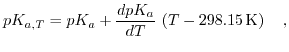
In order to further clarify the procedure, how to calculate the ionic strength and the different ion concentrations in the buffer, the procedure for a PBS will be presented. PBS contains orthosphoric acid
 and exhibits three dissociation reactions:
 |
(6.12) |
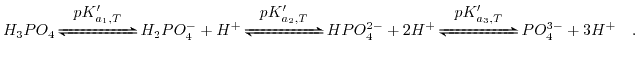
Table 6.1:
Parameters for the chosen phosphate buffer saline (PBS)[5].
|
|
Applying the Henderson-Hasselbach equation to (6.13) and utilizing charge conservation to gain the sodium concentration leads to the following set of equations:
![\begin{displaymath}\begin{array}{ccl} \left[\mathrm{H}_{3}\mathrm{PO}_{4}\right]...
...] - \xi_{3} \left[\mathrm{PO}_{4}^{3-}\right]\quad. \end{array}\end{displaymath}](img889.png) |
(6.13) |
Here,  ,
,  , and
, and  are the valencies of the
 ,
,
 , and
, and
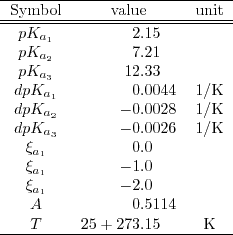
 , respectively, and the concentration of the PBS and the pH value in the bulk electrolyte is kept fixed. The iteration procedure given before with the values in Table 6.1 yields the ion concentrations depicted in Fig. 6.4, which illustrates the buffer ion concentrations and the ionic strength as a function of pH at
and
, respectively, and the concentration of the PBS and the pH value in the bulk electrolyte is kept fixed. The iteration procedure given before with the values in Table 6.1 yields the ion concentrations depicted in Fig. 6.4, which illustrates the buffer ion concentrations and the ionic strength as a function of pH at
and
 . The ionic strength rises strongly for small pH values (high
![$ \left[\mathrm{H}_{3}\mathrm{O}^{+}\right]$](img897.png) concentration) and high pH values (high
concentration) and high pH values (high
 concentration). Furthermore, the influence of the valence on the ionic strength is very pronounced due to the quadratic dependence in (6.9).
Figure 6.4:
The dependence of the concentrations for different ionic components and the ionic strength on the local pH.
|
|
Footnotes
- ... hybridized6.3
- Nucleic acid hybridization is the process of joining two complementary strands of DNA
Next: 6.3 Analytical Comparison of
Up: 6.2 Modeling BioFETs
Previous: 6.2.5 Debye-Hückel Model
T. Windbacher: Engineering Gate Stacks for Field-Effect Transistors
![\includegraphics[width=0.7\textwidth]{figures/pbs_pH.ps}](img899.png)