Next: 3.3 The Basic Semiconductor
Up: 3. The Box Integration
Previous: 3.1 The Poisson Equation
Subsections
3.2 The Diffusion Equation
In this section, the discretization of parabolic time-variant problems is described.
In its simplest representation, the right-hand side of the diffusion equation is time-invariant. Solving a diffusion problem the diffusion equation becomes time-variant. It describes the out-diffusion of matter, driven by its own concentration gradient.
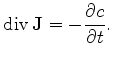
The diffusion flux
 can be written as
where  denotes the diffusion coefficient and
  is the concentration of the diffusing material.
Additionally, the conservation of material must be fulfilled
After insertion of (3.46) in (3.45), the diffusion equation can be reformulated as
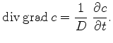 |
(3.47) |
As described in the previous section, this equation can be discretized as
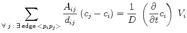 |
(3.48) |
The time derivative in this formula can be discretized by several methods. By the backward Euler method, the time derivative is approximated by [66]
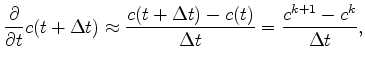 |
(3.49) |
with  the sampling interval. The discrete notation by backward Euler time discretization follows by
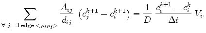 |
(3.50) |
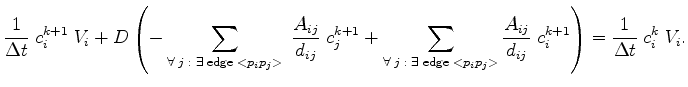
By separating the unknowns to the left-hand side, this expression becomes
In matrix notation, (3.51) can be written as
with
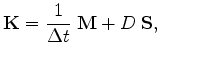 |
(3.53) |
The necessary boundary conditions for this parabolic equation can be handled as shown in the previous section. Also the requirements for an M-matrix (see Section 2.3) are satisfied. The conditions for
 can be handled as in the previous section and
 consists of positive diagonal entries only.
Additionally, an initial condition is required.
consists of positive diagonal entries only.
Additionally, an initial condition is required.
The initial concentration distribution at initial time  is defined as
 |
(3.60) |
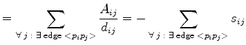
The discrete system is satisfied by the discrete formulation
 for all grid points for all grid points   |
(3.61) |
The concentration distributions
 can be computed by an sequential evaluation of .
Next: 3.3 The Basic Semiconductor
Up: 3. The Box Integration
Previous: 3.1 The Poisson Equation
J. Cervenka: Three-Dimensional Mesh Generation for Device and Process Simulation