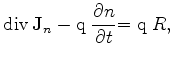
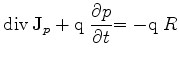
The classic drift-diffusion equations for electrons and holes read3.1
with
![]() the electron or hole current densities,
the electron or hole current densities, ![]() the electron or hole concentrations,
the electron or hole concentrations, ![]() and
and ![]() the carrier mobilities and diffusivities, and finally
the carrier mobilities and diffusivities, and finally
![]() the unit charge of the electron (positive).
These equations are connected via the recombination rate
the unit charge of the electron (positive).
These equations are connected via the recombination rate ![]()
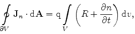 |
(3.67) |
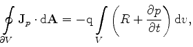 |
(3.68) |
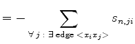
which must be satisfied for each Voronoi box of the tessellation. In the discrete form they can be rewritten as in (3.28)-(3.29)
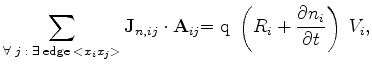 |
(3.69) |
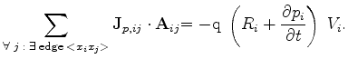 |
(3.70) |
 |
(3.71) |
 |
(3.72) |
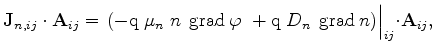
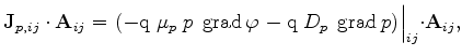
where, because of the inner product, only the components of the values along
![]() or along the edge
or along the edge
![]() remain
remain
with
 |
(3.75) |
 |
(3.76) |
 |
(3.77) |
 and and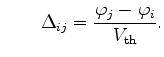 |
(3.78) |
| (3.79) |
 |
(3.80) |
 |
(3.81) |
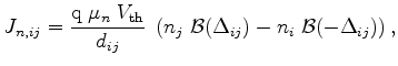
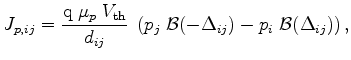
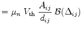
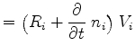
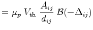
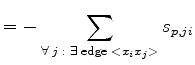
which results in the final discrete formulation of the semiconductor equations
| (3.82) | |
| (3.83) |
Here
 |
|
(3.84) | ||
 |
|
(3.85) | ||
 |
|
(3.86) | ||
 |
|
(3.87) | ||
 |
|
(3.88) | ||
 |
|
(3.89) |
This method is referred as Scharfetter-Gummel discretization [17][44][57].
The resulting expressions are linear equation systems in ![]() or
or ![]() where the boundary conditions can be set as in the previous sections. If calculating a non-stationary problem the time discretization can be performed as shown in Section 3.2.
where the boundary conditions can be set as in the previous sections. If calculating a non-stationary problem the time discretization can be performed as shown in Section 3.2.
The major difference to the field or diffusion equation is that the system matrices
![]() and
and
![]() are no longer symmetrical, because of
are no longer symmetrical, because of
![]() .
As the semiconductor equations for electrons (3.62) and holes (3.63) depend on the field equation (3.66) and this equation depends on the carrier concentrations itself, the whole differential equation system must be solved. While the dependency is nonlinear in
.
As the semiconductor equations for electrons (3.62) and holes (3.63) depend on the field equation (3.66) and this equation depends on the carrier concentrations itself, the whole differential equation system must be solved. While the dependency is nonlinear in ![]() , a recursive solution mechanism for solving this system is inevitable. As the coefficients of the matrices are influenced by
, a recursive solution mechanism for solving this system is inevitable. As the coefficients of the matrices are influenced by
![]() ,
a small potential change will influence the carrier concentrations exponentially, which influences the potential distribution itself.
A simple iterative approach, which evaluates each equation back-to-back and reinserts the updated values in the next iteration, does not deliver stable states. Newton or even specially damped Newton algorithms are required [5][67].
,
a small potential change will influence the carrier concentrations exponentially, which influences the potential distribution itself.
A simple iterative approach, which evaluates each equation back-to-back and reinserts the updated values in the next iteration, does not deliver stable states. Newton or even specially damped Newton algorithms are required [5][67].