


Next: 3.2 Structure of Relaxed
Up: 3. Strain Effects on
Previous: 3. Strain Effects on
Subsections
3.1 Theory of Elasticity
The property of solid materials to deform under the application of an external
force and to regain their original shape after the force is removed is referred
to as its elasticity. The external force applied on a specified area is known
as stress, while the amount of deformation is called the
strain. In this section, the theory of stress, strain and their
interdependence is briefly discussed.
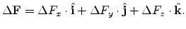
Imagine an object oriented in the cartesian coordinate system with a number of
forces acting on it, such that the vector sum of all the forces is zero. Take a
slice orthogonal to the
 -direction and define a small area on this
slice as
-direction and define a small area on this
slice as
 . Let the total force acting on this small area be
 |
(3.1) |
We can define the following scalar quantities.
 |
(3.2) |
The subscripts  and
and  in
in  refer to the plane and the force
direction, respectively. Similarly considering slices orthogonal to the
refer to the plane and the force
direction, respectively. Similarly considering slices orthogonal to the
 and
and
 -directions, we obtain
 |
(3.3) |
and
 |
(3.4) |
The scalar quantities can be arranged in a matrix form to yield the stress
tensor
 |
(3.5) |
The condition of static equilibrium implies
 .
.
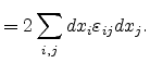
Figure 3.1:
Components of the stress tensor.
A body under elastic deformation experiences an internal restoring force. The
amount of deformation caused is called strain and the corresponding force, the
stress. Consider a pair of points at locations
 and
and
 which are deformed to locations
 and
and
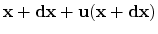 .
The absolute squared distance between the deformed points can be written as
.
The absolute squared distance between the deformed points can be written as
 |
(3.6) |
Assuming
 to be a small displacement, a Taylor expansion about the
point
gives the absolute squared distance as
to be a small displacement, a Taylor expansion about the
point
gives the absolute squared distance as
 |
(3.7) |
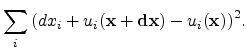
Since the first term in (3.7) denotes the original squared distance
between the points, the change in the squared distance becomes
 |
(3.8) |
![$\displaystyle = \sum_{i,j} dx_i\left[ { \left(\frac{\partial u_i}{\partial x_j}...
...\frac{\partial u_k}{\partial x_i }\frac{\partial u_k}{\partial x_j}}\right]dx_j$](img139.png) |
(3.9) |
 |
(3.10) |
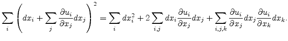
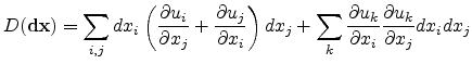
Here,
 denote the components of the strain tensor and are defined as
![$\displaystyle \varepsilon_{ij} = \frac{1}{2}\left[\frac{\partial u_i}{\partial ...
... \frac{\partial u_k}{\partial x_i }\frac{\partial u_k}{\partial x_j} } \right].$](img141.png) |
(3.11) |
Assuming that
 the
second order term in (3.11) can be neglected and the resulting tensor is
the
second order term in (3.11) can be neglected and the resulting tensor is
![$\displaystyle \varepsilon_{ij} = \frac{1}{2}\left[\frac{\partial u_i}{\partial x_j} + \frac{\partial u_j}{\partial x_i} \right].$](img143.png) |
(3.12) |
Note that in literature, engineering shear strain components,
 ,
are commonly used rather than the shear strain components described
by (3.12). The relation is,
,
are commonly used rather than the shear strain components described
by (3.12). The relation is,
 |
(3.13) |
Arranging the strain components (3.12) in matrix form gives the strain
tensor
 |
(3.14) |
The sign convention adopted for stress is that tensile stress causes an
expansion, whereas compressive stress causes a contraction.
The relation between stress and strain was first identified by Robert
Hook [Hook78]. Hook's law of elasticity is an approximation which states
that the amount by which a material body is deformed (the strain) is linearly
related to the force causing the deformation (the stress). The most general
relationship between stress and strain can be mathematically written as
 |
(3.15) |
Here,  is a fourth order elastic stiffness tensor comprising 81
coefficients. However, depending on the symmetry of the crystal the number of
coefficients can be reduced. For cubic crystals such as Si and Ge only three
unique coefficients
is a fourth order elastic stiffness tensor comprising 81
coefficients. However, depending on the symmetry of the crystal the number of
coefficients can be reduced. For cubic crystals such as Si and Ge only three
unique coefficients  ,
,  and
and  , exist. These coefficients
are known as the stiffness constants. To simplify the notations, the stress and
strain tensor can be written as vectors using the contracted notations
, exist. These coefficients
are known as the stiffness constants. To simplify the notations, the stress and
strain tensor can be written as vectors using the contracted notations
![$\displaystyle [Q_{xx},Q_{yy},Q_{zz},Q_{yz},Q_{xz},Q_{xy}] = [Q_1,Q_2,Q_3,Q_4,Q_...
...e{Q}}} = \ensuremath{{\underline{T}}}, \ensuremath{{\underline{\varepsilon }}},$](img151.png) |
(3.16) |
and the generalized Hook law in matrix form as
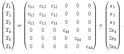 |
(3.17) |
Table 3.1:
Elastic stiffness constants  in GPa [Levinstein99] and
elastic compliance constants
in GPa [Levinstein99] and
elastic compliance constants  in
in  m
m /N.
/N.
Of practical interest is the strain arising from a certain stress
condition. The strain components can be obtained by inverting Hook's law and
utilizing the compliance coefficients,  .
.
 |
(3.18) |
The stiffness and compliance tensors are linked through the relation
 . Using this relation, the three independent compliance
coefficients can be calculated as
. Using this relation, the three independent compliance
coefficients can be calculated as
The compliance coefficients for Si and Ge, together with the stiffness
coefficients are listed in Table 3.1. It is interesting to note
that traditionally the stiffness coefficients are denoted by , while
the compliance coefficients are denoted by .
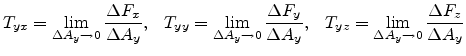
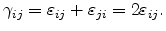
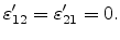
Figure 3.2:
Planes in the cubic system with the Miller indices marked.
The Miller indices, denoted as  ,
,  and
and  , are a symbolic vector
representation for the orientation of atomic planes and directions in a crystal
lattice. Defining three lattice vectors forming the lattice axes, any crystal
plane would intersect the axes at three distinct points. The Miller indices are
obtained by taking the reciprocal of the intercepted values. By convention,
negative indices are written with a bar over the indices. In Fig. 3.2,
three planes in the cubic system, along with their Miller indices are shown,
where the following nomenclature is adopted [Davies98].
, are a symbolic vector
representation for the orientation of atomic planes and directions in a crystal
lattice. Defining three lattice vectors forming the lattice axes, any crystal
plane would intersect the axes at three distinct points. The Miller indices are
obtained by taking the reciprocal of the intercepted values. By convention,
negative indices are written with a bar over the indices. In Fig. 3.2,
three planes in the cubic system, along with their Miller indices are shown,
where the following nomenclature is adopted [Davies98].
![$ [hkl]$](img175.png) represents a direction
represents a direction
-
 denotes equivalent directions
 represents a plane with the normal vector
 denotes equivalent planes
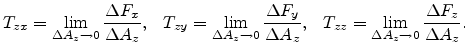
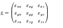
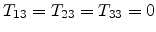
Figure 3.3:
Stress direction
![$ [x',y',z']$](img179.png) relative to the crystallographic
coordinate system
relative to the crystallographic
coordinate system ![$ [x,y,z]$](img180.png) .
.
It is often required to know the stress in the crystallographic coordinate system for a stress applied along
a general direction. Consider a generalized direction
in which the
stress is applied. The stress in the crystallographic coordinate system can be calculated using the
transformation matrix
 .
.
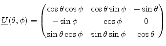 |
(3.19) |
Here  denotes the polar and
  the azimuthal angle of the stress
direction relative to the crystallographic coordinate system, as shown in
Fig. 3.3. The stress in the crystallographic coordinate system is then given by
the azimuthal angle of the stress
direction relative to the crystallographic coordinate system, as shown in
Fig. 3.3. The stress in the crystallographic coordinate system is then given by
 |
(3.20) |
Applying a non-zero stress of magnitude
 applied along the [100], [110]
and [111] directions, the stress tensors in the principal coordinate system
read, respectively
applied along the [100], [110]
and [111] directions, the stress tensors in the principal coordinate system
read, respectively
![$\displaystyle \ensuremath{{\underline{T}}}_{[100]} = \begin{pmatrix}P & 0 & 0 \...
...pmatrix}P/3 & P/3 & P/3 P/3 & P/3 & P/3 P/3 & P/3 & P/3 \end{pmatrix}.$](img188.png) |
(3.21) |
From (3.18), the corresponding strain tensors can be determined.
![$\displaystyle \ensuremath{{\underline{\varepsilon}}}_{[100]} = \begin{pmatrix}s...
...\cdot P & 0 & 0 0 & s_{12}\cdot P & 0 0 & 0 & s_{12}\cdot P \end{pmatrix}$](img189.png) |
(3.22) |
![$\displaystyle \ensuremath{{\underline{\varepsilon}}}_{[110]} = \begin{pmatrix}(...
...dot P/4 & (s_{11}+s_{12})\cdot P/2 & 0 0 & 0 & s_{12} \cdot P, \end{pmatrix}$](img190.png) |
(3.23) |
![$\displaystyle \ensuremath{{\underline{\varepsilon}}}_{[111]} = \begin{pmatrix}(...
... s_{44} \cdot P/6 & s_{44} \cdot P/6 & (s_{11}+2s_{12}) \cdot P/3 \end{pmatrix}$](img191.png) |
(3.24) |
For the case of epitaxially grown Si on SiGe, the in-plane strain
 is given by (2.1). Consider an interface (primed)
coordinate system, the
is given by (2.1). Consider an interface (primed)
coordinate system, the
 -axis of which is perpendicular to the Si/SiGe
interface. The strain tensor in this coordinate system can be written as
-axis of which is perpendicular to the Si/SiGe
interface. The strain tensor in this coordinate system can be written as
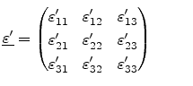 |
(3.25) |
with
 . Since epitaxial growth does not
produce any in-plane shear strain in the interface coordinate system, we have
. Since epitaxial growth does not
produce any in-plane shear strain in the interface coordinate system, we have
 |
(3.26) |
The other three independent strain components,
(
 ) can be determined as described
below [Hinckley90].
) can be determined as described
below [Hinckley90].
Since the strain is applied uniformly to the Si layer, all external stress
components in the vertical direction vanish,
 . Therefore, using Hook's law stated in (3.15) we have
 |
(3.27) |
where summation over repeated indices is implied. Expanding (3.27)
gives
 |
(3.28) |
which can be expressed in matrix form as
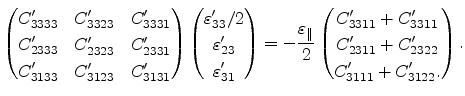 |
(3.29) |
The
 matrix elements can be determined from the elastic
stiffness tensor
matrix elements can be determined from the elastic
stiffness tensor
 through the relation,
 |
(3.30) |
where
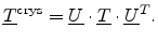
 denotes the transformation matrix in (3.19). Once the
matrix elements are known, (3.29) can be inverted to determine the
(
). Having determined the strain tensor in the
interface coordinate system, the tensor can be transformed to the principal coordinate systemusing
denotes the transformation matrix in (3.19). Once the
matrix elements are known, (3.29) can be inverted to determine the
(
). Having determined the strain tensor in the
interface coordinate system, the tensor can be transformed to the principal coordinate systemusing
 |
(3.31) |
Equations (3.29) and (3.31) can be solved to obtain the
strain tensor for epitaxial growth of Si on an arbitrarily oriented SiGe
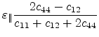
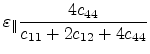
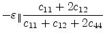
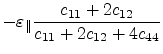
substrate. Table 3.2 lists the expressions for the
strain tensor components for the high-symmetry (001), (111) and (110) oriented
SiGe substrates.
Next: 3.2 Structure of Relaxed
Up: 3. Strain Effects on
Previous: 3. Strain Effects on
S. Dhar: Analytical Mobility Modeling for Strained Silicon-Based Devices


![\includegraphics[width=3.5in, angle=0]{figures/StressCoord3.eps}](img131.png)
![\includegraphics[width=6.5in,angle=0]{figures/miller.eps}](img173.png)
![\includegraphics[width=3.0in,angle=0]{figures/CoordTransform.eps}](img181.png)