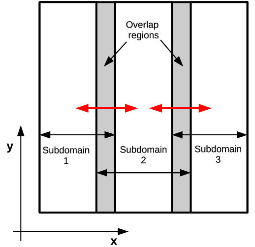
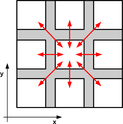
Figure 5.1: A uniform (a) slab- and (b) block-decomposition approach. Overlap areas shared by neighbouring subdomains are indicated in grey. The red
arrows indicate the communication links needed to transmit particles between subdomains.
The adoption of the domain decomposition approach requires consideration to be given to exactly how the domain decomposition is performed and how the process of annihilation is affected.
There are three design choices that must be made for the domain decomposition: i) the physical quantity to be decomposed, ii) the number of dimensions in this quantity to be decomposed and iii) the size of the subdomains. These three issues are discussed below.
The decomposition of the domain (phase space) can be either according to the spatial position or the wavevector (or a combination of both). The WBE presents a transport problem where the particles move in the domain (phase space) and have to be passed between subdomains, which necessitates a regular communication between the processes representing the subdomains. Moreover, in the signed-particle method (Chapter 3) particles are scattered/generated to/with new wavevectors, which can differ considerably from the original value/generating particle.
A decomposition of the k-space is not attractive from a performance point of view, because it is very likely that the new wavevector of the generated/scattered particle lies in a part of the k-space which is represented on another process and requires the particles to be transferred to this process. Considering the high particle generation rate (cf. Section 3.7.5) the additional communication required would be debilitating for parallel efficiency.
A decomposition of the spatial domain avoids such problems, since the position of particles change in a continuous, gradual fashion as they propagate; the position of newly generated particles also corresponds to that of the generating particle. As the particles propagate through the domain they are passed between neighbouring subdomains as they cross their boundaries. It should be pointed out that the boundaries between the subdomains are only of a computational nature and inconsequential to the mathematical formulation of the evolution, presented in Chapter 2.
For two- or three-dimensional problems one can choose the number of spatial dimensions to be partitioned. In the 2D case one has the choice between slab- and block-decomposition, which correspond to partitioning in one and two directions, respectively. Which decomposition method is best-suited depends on the computational resources and computational demands of the investigated problem; the physical behaviour of the problem also plays a deciding role. The case for 2D WEMC simulations is investigated here.
Slab-decomposition: A slab-decomposition splits the domain along a single direction (Figure 5.1a). The advantage of this approach is that the transfer of particles only has to be handled on two boundaries, thereby the communication is limited to only two other processes, which is advantageous for the parallel efficiency. Slab-decomposition will work well in simulation problems where there is a large degree of uniformity in one direction, e.g. the flow of particles is predominantly in one direction. In such a case, the domain is partitioned in the direction orthogonal to the flow. A judicious choice is important to achieve good load-balancing.
Since each subdomain/slab has a minimum width (one mesh cell), the maximum number of subdivisions/subdomains is limited. This places a maximum on the number of processes which can be used. Furthermore, the ’thinner’ the slabs are, the less particles can be accommodated in the subdomain – this gives rise to the situation where the computational load becomes too small in relation to the communication overhead incurred to transfer the particles between adjacent domains. Although these limits arise for all decomposition approaches, the slab-decomposition reaches these limits first. Nonetheless, the slab-decomposition method has been successfully applied to one- and two-dimensional Wigner Monte Carlo simulations [148, 149], as evidenced by the results in Section 5.5.
Block-decomposition: A partitioning in two spatial dimensions – a block decomposition – holds the promise to delay the onset of the limitations set out for the slab decomposition. Overall one attains greater granularity in the decomposition and can accommodate many more MPI processes. The number of communication links increases from 2 (slab-decomposition) to 8 per process since movement in the the diagonal directions must also be accounted for (Figure 5.1b). The additional communication channels which need to be set up with each time step introduce a significant overhead for the MPI communication back-end. Moreover, additional logic is required to identify to which subdomain particles have to be transferred to.
The computational load a process must handle is proportional to the number of particles in its subdomain. The domain decomposition approach allows a process to only treat the particles that are physically located in its subdomain. This complicates the task of load-balancing, since in a transport problem, by definition, there is a non-uniform distribution of particles moving about in the domain.
The size of the subdomains can be chosen such that the particles are more equally distributed (on average over time) between the processes, but this requires some heuristics as the optimal decomposition will differ considerably between different simulation problems. The situation is complicated by the fact that particles are also generated non-uniformly across the domain.
A possibility to make an a priori estimate of the particle distribution is to use the particle generation rate (assuming a time-independent potential is used; see Section 3.7.5) to weigh the size of the subdomains. The reasoning is that the most particles will end up being in the regions where there is the highest generation rate. This is only an approximation based on the assumption of a homogeneous initial distribution of particles across the entire domain. It is important to note that the distribution of the numerical particles does not correspond to the physical density, which takes the sign of the numerical particles into account.
The issue of load-balancing will not be treated further here; the remaining discussion and presented results (Section 5.5) assume a uniform decomposition of the spatial domain (and achieve reasonable scaling nonetheless).
Due to the domain decomposition, the portion of the phase-space associated with each process can be represented in the memory typically available for a single process (2 - 4GB). The annihilation step can be performed locally by each process for the particles in its subdomain – it is not required to perform the annihilation on a single process/node for the global ensemble. The only additional requirement is that the annihilation step must be performed amongst all the processes at a certain time step, i.e. if one process requires an annihilation step – as determined by its local growth prediction (Section 4.3.4) – all other processes should perform an annihilation, irrespective of whether it is required locally (according to the local growth prediction). This approach ensures that the global statistics (Wigner function) are not falsified. If an annihilation step would be performed in one sub-domain but not in the others, the number of particles representing the local distribution is reduced and thereby also its statistical weighting in the global ensemble.