
The Wigner function was introduced by Eugene Wigner in 1932 [52] with the motivation to add a quantum correction to the configuration of gases at low temperatures. He also derived the Wigner equation which describes the temporal evolution of the Wigner function. The Wigner formalism was originally deduced from the operator formalism. However, later a fully independent derivation was developed based on the Moyal bracket [53, 54].
The Wigner representation of an arbitrary physical quantity, like energy, is a function of the phase space coordinates. A mapping of the involved phase space functions to quantum mechanical operators is needed. Since quantum mechanical operators corresponding to position and momentum are not commutative, the ordering in which the variables appear matters in general and a simple correspondence principle is not sufficient to define a unique mapping. To remove the ambiguity in the mapping an additional ’rule’ is imposed, which defines the quantization scheme. Various quantization schemes have been proposed: normal ordering in which the position operator always precedes the momentum operator, anti-normal ordering (the converse) and fully symmetrized ordering (a mixture of both).
Another quantization scheme is the Weyl transform introduced by Hermann Weyl in 1927 [55]. The inverse mapping, from operators to functions, is known as the Wigner transform and is defined as
The Wigner transform is applied to the density operator and yields the Wigner function which amounts to a Fourier transform of the density matrix, expressed in the mean and difference of coordinates:

The Liouville-Von Neumann equation (1.34), introduced in Chapter 1, describes the evolution of the density matrix and is expressed here using the variables defined in (2.3):
Only a single differential operator remains – this is a convenience afforded by the assumption of a parabolic dispersion relation. However, the incorporation of more complicated bandstructures in the Wigner formalism has been approached by [56, 57].The Wigner transport equation is derived by applying the Wigner transform (2.1) to (2.6); the left-hand side (LHS) immediately yields the time derivative of the Wigner function. The transform of the first term on the right-hand side (RHS), related to the spatial derivatives, gives

 corresponds to a multiplication by ik in the transformed space. The transform of the remaining, potential-related terms on the RHS makes
use of the property
corresponds to a multiplication by ik in the transformed space. The transform of the remaining, potential-related terms on the RHS makes
use of the property = ∫
dr2δ
= ∫
dr2δ f
f to change the variable in the density matrix and yields
The property δ
to change the variable in the density matrix and yields
The property δ =
=  ∫
dk′eik′⋅
∫
dk′eik′⋅ then introduces a third integral such that (2.8) finally becomes
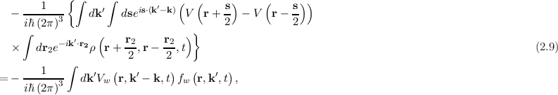
The Wigner function may assume both positive and negative values, which is a manifestation of the quantum uncertainty principle [44]. Nonetheless, a critical property of a probability distribution is retained:

 = exp
= exp , where A(t), a(t) and b(t) are a complex-valued matrix, vector and number,
respectively [58].
, where A(t), a(t) and b(t) are a complex-valued matrix, vector and number,
respectively [58].
The use of Wigner functions to describe quantum transport in semiconductor devices, which represent open quantum systems, is reviewed in [59]: the Wigner function of pure states is introduced in terms of generalized functions and, furthermore, it is proven that the mean value of an observable can be calculated as a weighted average of the mean values of the observable for the pure state. The convergence problems that arise when a potential difference occurs between the boundaries of the domain – as is the case for open quantum systems – can be treated by introducing a damping factor to the Wigner potential (2.10) [60].
The Wigner transport equation is a linear pseudo-differential equation. The Wigner equation (2.11) reduces to the Vlasov equation (collision-less Boltzmann
equation) for quadratic and linear potentials [52]. This can be readily shown by expressing the potential as a Taylor expansion in (2.11) [61]. Therefore, dynamic
quantum effects manifest themselves as derivatives of the potential of third-order and higher. In the semi-classical limit  the Vlasov equation is recovered,
regardless of the potential profile.
the Vlasov equation is recovered,
regardless of the potential profile.


