


Next: 2.4 Quantum Mechanical Effects
Up: 2. Simulation of Semiconductor
Previous: 2.2 Analytic MOSFET Approximations
Subsections
2.3 Carrier Generation and Recombination
Carrier generation is a process where electron-hole pairs are created by
exciting an electron from the valence band of the semiconductor to the
conduction band, thereby creating a hole in the valence band. Recombination is
the reverse process where electrons and holes from the conduction respectively
valence band recombine and are annihilated. In semiconductors several
different processes exist which lead to generation or recombination, the most
important ones are:
- photon transition or optical generation/recombination,
- phonon transition or Shockley-Read-Hall generation/recombination,
- Auger generation/recombination or three particle transitions, and
- impact ionization.
In thermal equilibrium the generation and recombination processes are in
dynamic equilibrium. When the system is supplied with additional energy, for
example through the absorption of photons or the influence of temperature,
additional carriers are generated. The most important generation/recombination
processes for the simulation of semiconductor devices are summarized in the
following.
2.3.1 Photon Transition
Figure 2.1:
Direct generation/recombination process. During photon assisted
recombination an electron from the conduction band re-combines with a hole in
the valence band. The excess energy is transferred to a photon. The reverse
process obtains its energy from radiation and generates an electron hole
pair.
|
|
The photon transition is a direct, band-to-band, generation/recombination
process. An electron from the conduction band falls back to the valence-band
and releases its energy in the form of a photon (light). The reverse process,
the generation of an electron-hole pair, is triggered by a sufficiently
energetic photon which transfers its energy to a valence band electron which is
excited to the conduction band leaving a hole behind. The photon energy for
this process has to be at least of the magnitude of the band-gap energy
 .
Figure 2.1 gives an overview of this process. The initial
electron/hole constellation is found in (a) while the constellation after the
generation/recombination process is found in (b).
.
Figure 2.1 gives an overview of this process. The initial
electron/hole constellation is found in (a) while the constellation after the
generation/recombination process is found in (b).
For these state changes in the semiconductor the energy and the momentum
have to be conserved. The energy is emitted or absorbed via a photon with the
energy
 |
(2.44) |
where  is Planck's constant and
  is the frequency of the emitted or
absorbed photon. However, as the momentum of a photon is very small no
momentum transfer is possible in the transition process. Therefore, only
direct band-to-band transitions are possible, where no change in momentum is
necessary. As silicon and germanium are indirect semiconductors and have their
valence band maximum and their conduction band minimum on different positions
in momentum space, direct transitions are very unlikely to occur and can in
most cases be neglected for those materials. In direct semiconductors like
GaAs, this effect is very important.
is the frequency of the emitted or
absorbed photon. However, as the momentum of a photon is very small no
momentum transfer is possible in the transition process. Therefore, only
direct band-to-band transitions are possible, where no change in momentum is
necessary. As silicon and germanium are indirect semiconductors and have their
valence band maximum and their conduction band minimum on different positions
in momentum space, direct transitions are very unlikely to occur and can in
most cases be neglected for those materials. In direct semiconductors like
GaAs, this effect is very important.
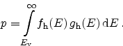
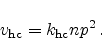
The process of carrier recombination is directly proportional to the amount of
available electrons and holes. By assuming the capture and emission rates
 and
and
 the recombination
and generation (
the recombination
and generation ( ) rates can be written as
 |
(2.45) |
 |
(2.46) |
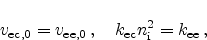
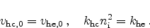
As the recombination and generation are balanced in thermal equilibrium, where

 |
(2.47) |
 |
(2.48) |
the total band-to-band recombination is calculated as the deviation from the
thermal equilibrium
 |
(2.49) |
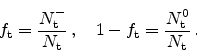
This process always strives for thermal equilibrium. For an excess
concentration of carriers
 and carrier recombination
dominates, while for low carrier densities
and carrier recombination
dominates, while for low carrier densities
 and
carrier generation prevails.
and
carrier generation prevails.
2.3.2 Phonon Transition
Figure 2.2:
Four sub-processes in the Shockley-Read-Hall
generation/recombination process. 1. electron capture, 2. hole capture,
3. hole emission, and 4. electron emission.
|
|
Another process is the generation/recombination by phonon emission. This
process is trap-assisted utilizing a lattice defect at the energy level
 within the semiconductor band-gap. The excess energy during recombination and
the necessary energy for generation is transferred to and from the crystal
lattice (phonon). A theory describing this effect has been established by
Shockley, Read, and Hall [7,8]. Therefore, the effect is
throughout the literature referenced as Shockley-Read-Hall (SRH)
generation/recombination. Four sub-processes are possible:
within the semiconductor band-gap. The excess energy during recombination and
the necessary energy for generation is transferred to and from the crystal
lattice (phonon). A theory describing this effect has been established by
Shockley, Read, and Hall [7,8]. Therefore, the effect is
throughout the literature referenced as Shockley-Read-Hall (SRH)
generation/recombination. Four sub-processes are possible:
- Electron capture. An electron from the conduction band is captured by an
empty trap in the band-gap of the semiconductor. The excess energy of
 is transferred to the crystal lattice (phonon emission).
- Hole capture. The trapped electron moves to the valence band and
neutralizes a hole (the hole is captured by the occupied trap). A phonon
with the energy
 is generated.
- Hole emission. An electron from the valence band is trapped leaving a
hole in the valence band (the hole is emitted from the empty trap to the
valence band). The energy necessary for this process is
.
- Electron emission. A trapped electron moves from the trap energy level
to the conduction band. For this process additional energy of the magnitude
has to be supplied.
These sub-processes are illustrated in Figure 2.2. (a) gives the
initial electron/hole constellation, the arrows schematically depict the
transition, and (b) gives the constellation after the sub-process.
Both, the recombination and the generation processes are two-step processes.
The sequential occurrence of sub-processes 1 and 2 leads to recombination of an
electron-hole pair. The excess energy of approximately the band-gap energy is
transferred to the crystal lattice via lattice vibrations, phonons. For the
SRH generation of an electron-hole pair sub-processes 3 and 4 are responsible.
Here external energy has to be supplied from the lattice.
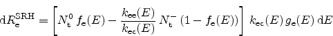
To derive an expression for the total recombination rate
 , rates for
every sub-process are introduced. Here, acceptor like traps are assumed, which
are neutral when empty and negatively charged when occupied by an electron.
The derivation for donor traps, which are neutral when occupied by an electron
and positively charged when empty, is similar and delivers the same result.
, rates for
every sub-process are introduced. Here, acceptor like traps are assumed, which
are neutral when empty and negatively charged when occupied by an electron.
The derivation for donor traps, which are neutral when occupied by an electron
and positively charged when empty, is similar and delivers the same result.
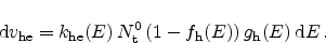
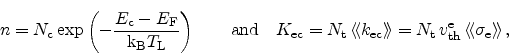
The electron capture rate  is proportional to the electron
concentration in the conduction band
is proportional to the electron
concentration in the conduction band  , the concentration of empty traps
 , and a proportionality constant
  . As the available
electrons are spread in energy in the conduction band, we must consider the
electron capture rate for different energies
. As the available
electrons are spread in energy in the conduction band, we must consider the
electron capture rate for different energies
 . With the energy dependent
distribution function for electrons
. With the energy dependent
distribution function for electrons
 and the density-of-states
 we get
 |
(2.50) |
This is the differential electron capture rate at energy
. The total
amount of conduction band electrons is
 |
(2.51) |
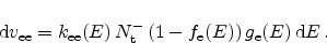
The hole capture rate  is proportional to the hole concentration
in the valence band
is proportional to the hole concentration
in the valence band  , the concentration of filled traps
 , and a
proportionality constant
, and a
proportionality constant  . Again, we consider the spread of the
holes in energy,
. Again, we consider the spread of the
holes in energy,
 |
(2.52) |
Here,
 is the distribution function for holes and
 the
density-of-states. The total amount of holes in the valence band is
the
density-of-states. The total amount of holes in the valence band is
 |
(2.53) |
The hole emission rate  is proportional to the concentration of
empty traps, the proportionality constant
is proportional to the concentration of
empty traps, the proportionality constant  ,
,
 |
(2.54) |
And finally the electron emission rate  is proportional to the
concentration of filled traps and the proportionality constant
is proportional to the
concentration of filled traps and the proportionality constant 
 |
(2.55) |
The total trap concentration
 is
is
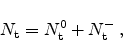 |
(2.56) |
and the fraction of occupied traps
 is given by
 |
(2.57) |
With these definitions the net recombination rate for electrons becomes
 |
(2.58) |
In thermal equilibrium (
 ) the net generation equals
zero, which means that the respective capture and emission rates for electrons
and holes must be equal
) the net generation equals
zero, which means that the respective capture and emission rates for electrons
and holes must be equal
 |
(2.59) |
From (2.58) we obtain using (2.59)
 |
(2.60) |
In thermal equilibrium
 is given by Fermi-Dirac statistics
 |
(2.61) |
with the property
 |
(2.62) |
The ratio (2.60) then calculates as
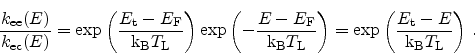 |
(2.63) |
Using (2.63) we can further develop (2.58)
 |
(2.64) |
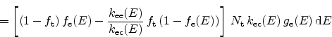 |
(2.65) |
 |
(2.66) |
![\begin{displaymath}=\left[ 1 - \exp \left( \frac{\ensuremath{E_\textrm{t}}-
\en...
...emath{\textrm{k$_\textrm{B}$}}T_\textrm{L}} \right) \right] \end{displaymath}](img215.png) |
(2.67) |
 |
(2.68) |
 |
(2.69) |
with the trap's quasi Fermi energy
 .
.
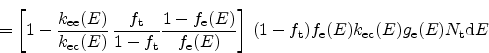
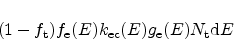
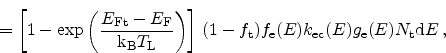
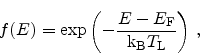
Integrating over all possible electron energies gives the total electron
recombination rate
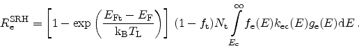 |
(2.70) |
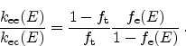
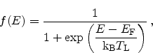
Typically a capture cross section
 is introduced to rewrite
 as
as
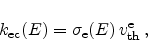 |
(2.71) |
with the thermal velocity for electrons
 |
(2.72) |
resulting in
|
(2.73) |
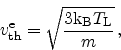
For non-degenerate semiconductors near equilibrium a Maxwell-Boltzmann
distribution can be assumed
 |
(2.74) |
and one obtains for the integral in (2.73)
 |
(2.75) |
with the properties
 |
(2.76) |
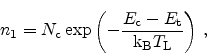
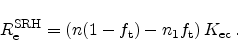
where
 is the effective density-of-states for electrons we have
 |
(2.77) |
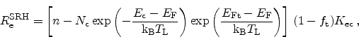
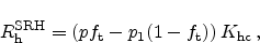
and
![\begin{displaymath}
\ensuremath{R^\textrm{SRH}_\textrm{e}}= \left[ n (1-\ensure...
...uremath{f_\textrm{t}}\right] \ensuremath{K_\textrm{ec}} .
\end{displaymath}](img229.png) |
(2.78) |
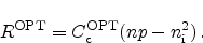
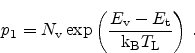
Introducing the auxiliary quantity
 |
(2.79) |
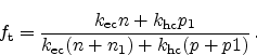
we finally get for the electron recombination rate
 |
(2.80) |
Analogously the hole recombination rate can be obtained as
 |
(2.81) |
by introducing
 |
(2.82) |
In transient simulations the capture and emission rates are not equal.
Therefore, no further simplifications are possible and an additional equation
has to be solved for each trap
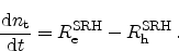 |
(2.83) |
This increases the computational effort significantly but is necessary for
example to simulate the charge pumping effect (Section 4.1).
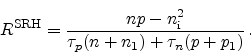
In the stationary case electrons and holes always act in pairs thus the
recombination rates for electrons and holes are equal,
 |
(2.84) |
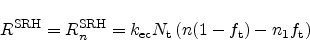
Therefore, we can calculate
from (2.80) and (2.81) as
 |
(2.85) |
Using this expression for the total recombination rate we get
 |
(2.86) |
 |
(2.87) |
 |
(2.88) |
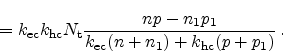
It is very common to introduce carrier lifetimes for electrons and holes
 and
and

 |
(2.89) |
By using the capture cross sections for electrons and holes,
 and
and
 , and the thermal velocities
 and
and

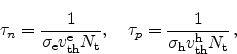 |
(2.90) |
we come to the final formulation of the Shockley-Read-Hall model for carrier
generationrecombination
 |
(2.91) |
Regarding the efficiency of trap centers it can be seen that the energy
transfer necessary for generationrecombination is always approximately
the band-gap energy, no matter where the trap energy level is. The reason is
that carriers are transferred from one energy band-edge to the trap level and
further to the other band-edge, giving in total the band-gap energy. But when
the two sub processes capture and emission are considered, it can be seen that
the further the trap energy is away from the mid-gap energy, the higher is the
necessary energy for either capture or emission and the lower for the
respective other process. The highest energy in this two-step process is
always limiting the total generation/recombination. When the trap is located
in the middle of the band-gap, the resulting energy barrier height is half the
band-gap energy. As the trap is moved away from the mid-gap energy, the
limiting energy barrier is increased and the probability of
generation/recombination is reduced.
Impurities used for doping semiconductors are usually energetically situated
very close to either the valence or the conduction band in order to be
effective doping centers. They are therefore not very effective for carrier
generation/recombination and are called ``shallow'' traps. ``Deep'' traps on
the other hand are located close to the mid-gap which can be used to
artificially increase the carrier generation or recombination.
For the investigation of NBTI the generation and recombination mechanisms at
the silicondielectric interface are of major importance
(Chapter 3). The Shockley-Read-Hall generation/recombination
mechanism can also be applied to traps at the interface, which is for example
obligatory for the simulation of the charge pumping effect
(Section 4.1).
The derivation for recombination at surface traps is similar to the derivation
for bulk traps. The major difference is the different unit for interface traps
![$[\ensuremath{N_\textrm{it}}]=1/\mathrm{cm}^2$](img249.png) and the resulting unit for the surface recombination
velocity
and the resulting unit for the surface recombination
velocity
![$[\ensuremath{R^\textrm{SRH}_\textrm{it}}]=1/\mathrm{cm}^2 \mathrm{s}$](img250.png) .
.
As described in detail in Section 3.1.1, interface traps are not located
on discrete energy levels but distributed in the band-gap instead. When
accounting for the trap density-of-states
 , we get for the
interface trap concentration
, we get for the
interface trap concentration
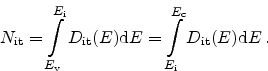 |
(2.92) |
The interface trap recombination rate is then obtained as
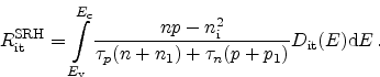 |
(2.93) |
Figure 2.3:
Four sub-processes in the Auger generation/recombination mechanism.
1. electron capture, 2. hole capture, 3. electron emission, and 4. hole
emission.
|
|
In the direct band-to-band Auger mechanism three particles are involved.
During generation an electron hole pair is generated consuming the energy of a
highly energetic particle. In the opposite process, when an electron hole pair
recombines, the excess energy is transferred to a third particle. In detail
the four possible processes are as follows:
- Electron capture. An electron from the conduction band moves to the
valence band neutralizing a hole in the valence band. The excess energy is
transferred to an electron in the conduction band.
- Hole capture. Again, an electron from the conduction band moves to the
valence band and recombines with a valence hole. The excess energy is, in
contrast to Process 1, transferred to another hole in the valence band.
- Electron emission. A highly energetic electron from the conduction band
transfers its energy to an electron in the valence band. The valence
electron moves to the conduction band generating an electron hole pair.
- Hole emission. A highly energetic hole from the valence band transfers its
energy to an electron in the valence band which is then excited to the
conduction band generating an electron hole pair.
These sub-processes are illustrated in Figure 2.3. (a) gives the
initial electron/hole constellation, the arrows schematically depict the
transition, and (b) gives the constellation after the sub-process.
As for the Shockley-Read-Hall effect a model can be derived by setting up rates
for the four processes.
For electron capture two electrons in the conduction band and one hole in the
valence band are necessary. Using as the rate constant, the
electron capture rate becomes
 |
(2.94) |
Analogical for hole capture where two holes and one electron are involved
evaluates as
 |
(2.95) |
For electron and hole emission only one respective carrier is necessary
 |
(2.96) |
 |
(2.97) |
In thermal equilibrium the respective capture and emission rates are in
equilibrium, and therefore
 |
(2.98) |
 |
(2.99) |
This leads us to the final model for the Auger recombination rate

 |
(2.100) |
Although the Auger mechanism is microscopically exactly the same as the
mechanism during impact ionization described in the next section, the energy
source is completely different. Whereas impact ionization relies on high
current density, only a very large carrier density is of importance for Auger
generation/recombination, as can be seen in the final formulation of
(2.100).
2.3.4 Impact Ionization
Figure 2.4:
Impact ionization and avalanche multiplication. An energetic
electron donates its energy to the generation of an electron hole pair. The
newly generated electron can, due to the high electric field, obtain high
energy and generate further carriers, leading to avalanche multiplication.
|
|
Impact ionization is a pure generation process. Microscopically it is exactly
the same mechanism as the generation part of the Auger process: a highly
energetic carrier moves to the conduction or valence band, depending on the
carrier type, and the excess energy is used to excite an electron from the
valence band to the conduction band generating another electron hole pair. The
major difference is the cause of the effect. While it is purely the carrier
concentration in the Auger mechanism, for impact ionization it is the current
density.
Two partial processes can be distinguished:
- Electron emission. A highly energetic electron from the conduction band
transfers its energy to an electron in the valence band. The valence
electron moves to the conduction band generating an electron hole pair.
- Hole emission. A highly energetic hole from the valence band transfers
its energy to an electron in the valence band which is then excited to the
conduction band generating an electron hole pair.
Figure 2.4 depicts the effect of impact ionization and avalanche
multiplication. The leftmost, highly energetic, electron excites a new
electron/hole pair which gains energy and generates further carriers. The
result is an avalanche multiplication of carrier generation.
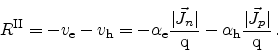
As already mentioned, the generation rates are modeled proportional to the
current densities
 and
and
 and can be written as:
 |
(2.101) |
 |
(2.102) |
with the ionization rates for electrons and holes,
 and
and
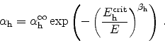
 . These rates are typically described with an exponential
dependence upon the electric field component in the direction of the current
flow
. These rates are typically described with an exponential
dependence upon the electric field component in the direction of the current
flow  . With the critical electric fields for electrons and holes,
 and
and
 , and the
ionization rates at infinite field,
, and the
ionization rates at infinite field,
 and
and
 , the ionization rates evaluate as
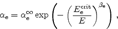 |
(2.103) |
 |
(2.104) |
Here,
 and
and
 are additional model
parameters, which are in the range of 1-2. The total impact ionization rate
is now found as
are additional model
parameters, which are in the range of 1-2. The total impact ionization rate
is now found as
 |
(2.105) |
The impact ionization rate does not actually depend on the local electric field
but on the carrier temperature and, thus, on the high-energy tail of the
distribution function. Therefore, the model is not very accurate, especially
in small devices. Carriers need to travel a certain distance in the high
electric field in order to gain energy. For the exact modeling semiconductor
device equations of higher order are necessary.
Next: 2.4 Quantum Mechanical Effects
Up: 2. Simulation of Semiconductor
Previous: 2.2 Analytic MOSFET Approximations
R. Entner: Modeling and Simulation of Negative Bias Temperature Instability
![\includegraphics[width=10cm]{figures/photon-emission}](img158.png)
![\includegraphics[width=16cm]{figures/srh-processes}](img174.png)
![\includegraphics[width=16cm]{figures/auger-processes}](img254.png)
![\includegraphics[width=8cm]{figures/ii-processes}](img263.png)