For the initialization of the LS function, triangles must be checked for possible intersections with grid lines (see Section 4.1.1). In the following, a robust line-triangle intersection test is presented. If the line intersects the triangle, the intersection point is also calculated. The following approach ensures that, if a line close to an edge fails the intersection test due to numerical errors, the test will succeed for another triangle, which is adjacent to the same edge. Hence, if a surface is given as a triangulation, cases, where the line fails all intersection tests, although it intersects the surface, are avoided.
A triangle with vertices
![]() ,
,
![]() , and
, and
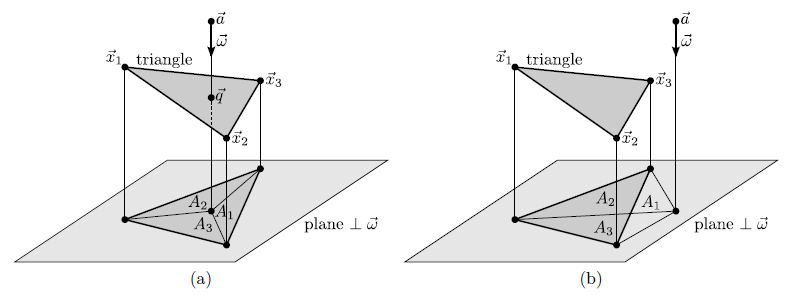
![]() is intersected by a line defined by point
is intersected by a line defined by point ![]() and unit vector
and unit vector
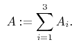
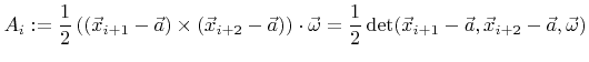
![]() , if the (signed) areas
, if the (signed) areas
|
To guarantee that lines close to an edge succeed the intersection test for any of the two adjacent triangles, the numerical evaluation of (A.1) must preserve the anticommutativity with respect to
![]() and
and
![]() . However, due to numerical errors this is usually not the case. For example, the numerical result of
. However, due to numerical errors this is usually not the case. For example, the numerical result of
![]() is not necessarily the same as that of
is not necessarily the same as that of
![]() with opposite sign [100]. To overcome this problem, the two vectors
with opposite sign [100]. To overcome this problem, the two vectors
![]() and
and
![]() in (A.1) are compared using an order relation, such as lexicographical comparison. If
in (A.1) are compared using an order relation, such as lexicographical comparison. If
![]() is larger than
is larger than
![]() , the two vectors are swapped, and the final result of (A.1) is inverted. This technique ensures the anticommutativity in (A.1).
, the two vectors are swapped, and the final result of (A.1) is inverted. This technique ensures the anticommutativity in (A.1).
Once the areas ![]() are determined and the intersection test is positive, the intersection point
are determined and the intersection test is positive, the intersection point ![]() can be obtained by
can be obtained by
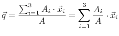 with
with