B.1 Setup of the Polynomial

Inserting the ray parameterization (B.1) into (B.4) leads to a polynomial of order ${D}$

$$\sum_{i=0}^{D}{C}_k t^k.$$ (B.8)

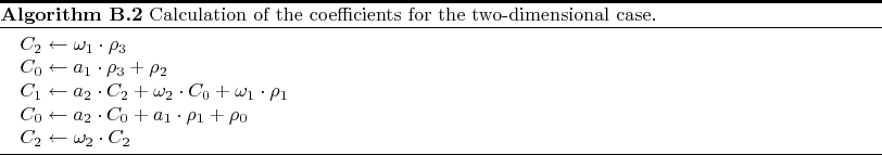
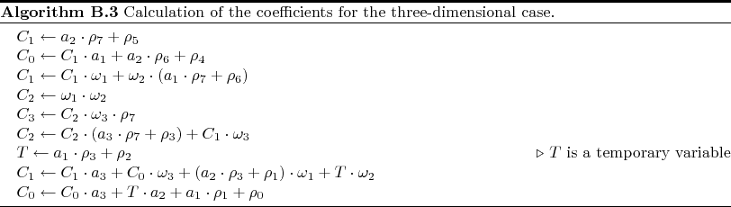
The calculation of the coefficients ${C}_k$ described in the literature [69,74,88,119] is not optimal in terms of the number of required multiplications. Therefore, optimized algorithms, Algorithm B.2 and Algorithm B.3, have been developed for the two- and three-dimensional cases, respectively. There, $\rho_k$ denotes the $k$ -th element of the multi-linear polynomial coefficients $\rho_{\vec{\beta}}$ , if they are sorted in lexicographical order. For example, $\rho_3$ corresponds to $\rho_{\left(1,1,0\right)}$ in the three-dimensional case.