1.4.1 Fast Level Set Framework

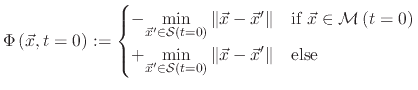
The presented simulations and models function fully within the process simulator presented in [50]. The LS method is utilized in order to describe the top surface of a semiconductor wafer as well as the interfaces between different materials. The LS method describes a movable surface $\mathcal{S}\left(t\right)$ as the zero LS of a continuous function $\Phi\left(\vec{x},t\right)$ defined on the entire simulation domain,

$\displaystyle \mathcal{S}\left(t\right)=\left\{ \vec{x}:\Phi\left(\vec{x},t\right)=0\right\}.$

(1)

The continuous function $\Phi\left(\vec{x},t\right)$ is obtained using a signed distance transform

$\displaystyle \Phi\left(\vec{x},t=0\right):=\begin{cases}-{\displaystyle \min_{... ...(t=0\right)}}\left\Vert \vec{x}-\vec{x}'\right\Vert & \textrm{else} \end{cases}$

(2)

where $\mathcal{M}$ is the material described by the LS surface $\Phi\left(\vec{x},t=0\right)$ . The implicitly defined surface $\mathcal{S}\left(t\right)$ describes a surface evolution, driven by a scalar velocity $V\left(\vec{x}\right)$ , using the LS equation

$\displaystyle \cfrac{\partial\Phi}{\partial t}+V\left(\vec{x}\right)\left\Vert \nabla\Phi\right\Vert =0.$

(3)

In order to find the location of the evolved surface, the velocity field $V\left(\vec{x}\right)$ must be found. When simulating various processes, both traditional [50] and those covered in this work, the velocities can be a scalar value or a value calculated using the technique described in Section 1.4.2.

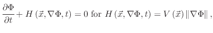
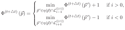
The LS equation can be solved using numerical schemes developed for the solution of Hamilton-Jacobi equations, since the LS equation belongs to the class of Hamilton-Jacobi equations, given by

$\displaystyle \cfrac{\partial\Phi}{\partial t}+H\left(\vec{x},\nabla\Phi,t\righ... ...c{x},\nabla\Phi,t\right)=V\left(\vec{x}\right)\left\Vert \nabla\Phi\right\Vert,$

(4)

where

denotes the Hamiltonian. The LS equation can then be solved using finite difference schemes such as the Euler method [176], the Upwind scheme, based on the Engquist-Osher scheme [49], or the Lax-Friedrichs Scheme for non-convex Hamiltonians [185]. Another advantage of using the LS method is that calculations of geometric variables such as the surface normal or the curvature are available directly from the implicit surface representation. The normal at a point $\vec{x}$ on the surface is given by

$\displaystyle \vec{n}\left(\vec{x}\right)=\cfrac{\nabla\Phi}{\left\Vert \nabla\Phi\right\Vert }$

(5)

and the curvature is

$\displaystyle \kappa\left(\vec{x}\right)=\nabla\vec{n}\left(\vec{x}\right)=\nabla\cfrac{\nabla\Phi}{\left\Vert \nabla\Phi\right\Vert }.$

(6)

1.4.1.1 Sparse Field Method

The initially proposed LS method uses a LS function which is defined on the entire simulation domain. However, memory requirements for the discretization of the LS function scale with domain size. Therefore, alternatives were proposed in the form of the narrow band method, where only a few layers around the LS surface are active grid points, and sparse field method [226], where a single layer of active grid points are considered for time integration. The steps required to implement the utilized process simulator are described by [50]

Update the LS values of all active grid points $\vec{p} \in \mathcal{L}^{(t)}_0$ in time using a finite difference scheme. $\mathcal{L}^{t}_0$ represents the most inner layer of grid points nearest to the LS surface.
If there are two neighboring points $\vec{p}_-,\vec{p}_+ \in \mathcal{L}^{(t)}_0$ for which $\Phi\left(\vec{p}_{-}\right)<-\cfrac{1}{2}$ and $\Phi\left(\vec{p}_{+}\right)>-\cfrac{1}{2}$ the absolute LS value for both points are reduced to $-\cfrac{1}{2}$ and $\cfrac{1}{2}$ respectively.
The LS values of all grid points $\vec{p}\in\mathcal{L}^{(t)}_i$ belonging to outside layers , where $i=\pm 1,\pm 2,...$ are updated

$\displaystyle \Phi^{\left(t+\triangle t\right)}\left(\vec{p}\right)=\begin{case... ...ft(t+\triangle t\right)}\left(\vec{p}\,'\right)-1 & \text{ if}\ i<0 \end{cases}$ (7)
Finally, the layers $\mathcal{L}_{i}^{\{(t+\triangle t)\}}$ which contain active grid points in the next time step are determined.

1.4.1.2 H-RLE Data Structure

For the calculation of finite difference schemes, the LS framework needs only to store the LS values of defined grid points, which is the union of all active grid points and their neighbors. The HRLE data structure [83] is used in order to store the discretized LS function. This structure is a hybrid between the DTG and the RLE data structures. It combines the linear scaling memory requirements of the DTG with adaptation to all grid directions. The HRLE data structure is organized hierarchically, similar to the DTG, where in place of storing a sequence of defined grid points, RLE is applied. Therefore, the structure is capable of storing the sign of the LS function for undefined grid points, while having the memory consumption of a DTG structure. The details of the implementation and examples showing the differences between the different data structures are described in [50]

1.4.1.3 Multiple Material Regions

Another important aspect of the LS framework is the ability to describe multiple LS surfaces for different material regions. The definition of different material regions in the LS framework was designed with etching processes in mind. When simulating traditional semiconductor processes, deposition is usually performed on the top layer, making masking not necessary. However, etching is almost always a masked process. Therefore the mask must be identifiable within the multi-LS framework. Figure 1.2 shows how material regions are labeled, resulting in an etch-friendly environment. When material $\mathcal{M}_2$ needs to be etched, with $\mathcal{M}_1$ serving as a mask, the LS defined by $\Phi_2$ needs to be moved in the negative direction, but only at the locations where it is not touching the $\Phi_1$ surface.

Figure 1.2: Numbering of material regions in (a) leads to the Level Set description in (b).

$\includegraphics[width=0.3\linewidth]{chapter_introduction/figures/LS_labels_vol.eps}$	$\includegraphics[width=0.3\linewidth]{chapter_introduction/figures/LS_labels.eps}$
(a) Material regions labeling	(b) Materials LS representation

If material $\mathcal{M}_2$ is deposited or grown with $\mathcal{M}_1$ serving as a mask, it is evident that the LS definitions from Figure 1.2b will result in the material deposition on top of $\mathcal{M}_1$ , which is undesired. Therefore, when $\Phi_2$ needs to be grown with $\Phi_1$ serving as a mask, as is the case with the oxidation process, the LS definition and numbering must be changed.

L. Filipovic: Topography Simulation of Novel Processing Techniques