3.5.2 The GUNDLACH Method

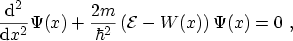
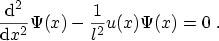
The GUNDLACH method [137] provides an analytical solution of SCHRÖDINGER's equation for a linear energy barrier. The one-dimensional time-independent SCHRÖDINGER equation in this case reads

$$\frac{\ensuremath {\mathrm{d}}^2}{\ensuremath {\mathrm{d}}x^2} \Psi(x) + \frac{2m}{\hbar^2} \left({\mathcal{E}}- W(x) \right) \Psi(x) = 0 \ ,$$ (3.61)

with the linear potential energy $W(x)$ between the points $x_0$ and $x_1$, $W_0 = W(x_0)$, and $W_1 = W(x_1)$,

$$W(x) = W_0 + (x - x_0) \frac{W_1 - W_0}{x_1 - x_0}$$ (3.62)

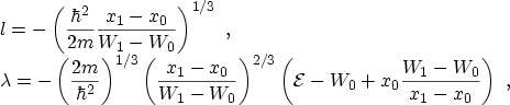
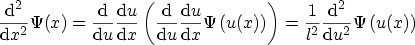
for $x_0 < x < x_1$. Using the abbreviations

$$\begin{array}{l} \displaystyle l = - \left( \frac{\hbar ^ 2}{... ...}- W_0 + x_0 \frac{W_1 - W_0}{x_1 - x_0}\right) \ , \end{array}$$ (3.63)

and $u(x) = \lambda - x / l$, expression (3.61) turns into

$$\frac{\ensuremath {\mathrm{d}}^2}{\ensuremath {\mathrm{d}}x^2} \Psi(x) -\frac{1}{l^2} u(x) \Psi(x) = 0 \ .$$ (3.64)

With

$$\frac{\ensuremath {\mathrm{d}}^2}{\ensuremath {\mathrm{d}}x^2} \P... ...c{\ensuremath {\mathrm{d}}^2}{\ensuremath {\mathrm{d}}u^2}\Psi\left(u(x)\right)$$ (3.65)

SCHRÖDINGER's equation evolves into the AIRY^3.7 differential equation

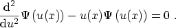$$\frac{\ensuremath {\mathrm{d}}^2}{\ensuremath {\mathrm{d}}u^2} \Psi\left(u(x)\right) - u(x) \Psi\left(u(x)\right) = 0 \ .$$ (3.66)

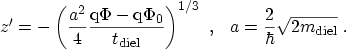
The solutions of this differential equation are the AIRY functions $\ensuremath{\mathrm{Ai}}\left(u(x)\right)$ and $\ensuremath{\mathrm{Bi}}\left(u(x)\right)$ [138], which are depicted in Fig. 3.10 together with their derivatives. The wave functions consist of linear superpositions of these AIRY functions

$$\Psi(x) = A \ensuremath{\mathrm{Ai}}\left(u(x)\right) + B \ensuremath{\mathrm{Bi}}\left(u(x)\right) \ ,$$ (3.67)

where the function $u(x)$ is given as

$$u(x) = - \left( \frac{2m}{\hbar^2} \right)^{1/3} \left( \frac{x_1 - x_0}{W_1 - W_0} \right)^{2/3} \left({\mathcal{E}}- W(x) \right) \ .$$ (3.68)

Figure 3.10: The AIRY functions Ai and Bi and their derivatives.

Assuming a constant electron mass in the dielectric, GUNDLACH derives an expression for the transmission coefficient

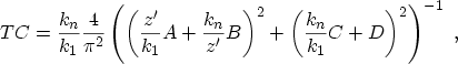$$TC = \frac{k_n}{k_1} \frac{4}{\pi^2}\left( \left( \frac{z'}{k_1} ... ...frac{k_n}{z'}B\right)^2 + \left( \frac{k_n}{k_1}C + D\right)^2 \right)^{-1} \ ,$$ (3.69)

where the abbreviations

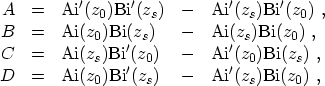$$\begin{array}{rclcl} A &=& \ensuremath{\mathrm{Ai}}'(z_0) \en... ...mathrm{Ai}}'(z_s) \ensuremath{\mathrm{Bi}}(z_0) \ , \end{array}$$ (3.70)

have been used and the symbols $z_0$, $z_s$, and $z'$ are given by

$$\begin{array}{cc} z_0 = (\ensuremath {\mathrm{q}}\Phi_0 - {\m... ...emath {\mathrm{q}}(\Phi - \Phi_0)}\right)^{2/3} \ , \end{array}$$ (3.71)

and

$$\begin{array}{cc} z' = -\left( \displaystyle\frac{a^2}{4} \di... ...{2}{\hbar} \sqrt{2\ensuremath{m_\mathrm{diel}}} \ . \end{array}$$ (3.72)

The symbols $\ensuremath {\mathrm{q}}\Phi$ and $\ensuremath {\mathrm{q}}\Phi_0$ denote the two edges of the energy barrier as shown in Fig. 3.9. The GUNDLACH method is frequently used in the literature [121,139] and implemented in device simulators. Numerical problems may occur for flat barriers ( $\Phi \approx \Phi_0$) due to the exponential increase of the AIRY functions $\ensuremath{\mathrm{Bi}}$ and $\ensuremath{\mathrm{Bi}}'$ for positive arguments. In practical implementations the values of $z_0$ and $z_s$ have been bounded to values below $\approx 200$ to avoid floating point overflow.

A. Gehring: Simulation of Tunneling in Semiconductor Devices