3.8.2.1 Capture and Emission Probabilities

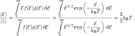
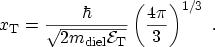
The tunneling model is based on a two-step tunneling process via traps in the dielectric which incorporates energy loss by phonon emission [219]. Fig. 3.17 shows the basic two-step process of an electron tunneling from a region with higher FERMI energy (the cathode) to a region with lower FERMI energy (the anode). To avoid integration in energy, the initial electron energy is assumed to be located at the average kinetic energy, which, for the parabolic dispersion relation (3.1) and the MAXWELLian distribution (3.20), is

$$\frac{\langle {\mathcal{E}}\rangle}{\langle 1 \rangle} = \frac {\... ...right) \,\ensuremath {\mathrm{d}}{\mathcal{E}}} = \frac{3}{2}{\mathrm{k_B}}T\ .$$ (3.130)

During the capture process ( $\ensuremath{W_\mathrm{c}}$), the difference in total energy between the initial and final state is released by means of phonon emission ( $\hbar \omega$). An electron captured by a trap can then be emitted into the anode ( $\ensuremath{W_\mathrm{e}}$).

The rate with which an electron with energy ${\mathcal{E}}$ is captured by a trap located at position $x$ and energy ${\mathcal{E}}^\prime$ is given by [221]

$$\ensuremath{W_\mathrm{c}}(x,{\mathcal{E}}^{\prime},{\mathcal{E}})... ...c{\displaystyle \Delta {\mathcal{E}}}{\displaystyle 2{\mathrm{k_B}}T}\right)\ .$$ (3.131)

Here, $S$ is the HUANG-RHYS factor which characterizes the electron-phonon interaction [222], $\hbar \omega$ is the energy of the phonons involved in the transitions, $\ensuremath{\Delta {\mathcal{E}}}={\mathcal{E}}-{\mathcal{E}}^\prime$, and $P=\ensuremath{\Delta {\mathcal{E}}}/ \ensuremath{\hbar\omega}$ is the number of phonons emitted due to this energy difference. In the simulations the value of $S\ensuremath{\hbar\omega}$ was used as fitting parameter.

The population of phonons $\ensuremath{f_\mathrm{P}}$ is given by the BOSE^3.11-EINSTEIN^3.12 statistics

$$\ensuremath{f_\mathrm{P}}=\left( \exp \left( \frac{\hbar \omega }{k_{B}T}\right) -1\right) ^{-1}\ .$$ (3.132)

Figure 3.17: The trap-assisted tunneling process.

The function $I_P(\xi)$ is the modified BESSEL^3.13 function of order $P$, with

$$\xi =2S\sqrt{\ensuremath{f_\mathrm{P}}(\ensuremath{f_\mathrm{P}}+1)} \ .$$ (3.133)

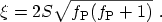
The term $\left\vert\ensuremath{V_\mathrm{e}}\right\vert^{2}$ in (3.131) denotes the transition matrix element which is calculated by an integration over the trap cube [220]

$$\ensuremath{\left\vert\ensuremath{V_\mathrm{e}}\right\vert^{2}}=5... ...ensuremath{x_\mathrm{T}}/ 2} \vert\Psi(x)\vert^2 \,\ensuremath {\mathrm{d}}x\ .$$ (3.134)

In this expression $x_\mathrm{T}$ denotes the side length of the trap cube, estimated as

$$\ensuremath{x_\mathrm{T}}= \frac{\hbar }{\sqrt{2\ensuremath{m_\ma... ...}\ensuremath{{\mathcal{E}}_\mathrm{T}}}} \left( \frac{4\pi }{3}\right)^{1/3}\ .$$ (3.135)

The symbol ${\mathcal{E}}_\mathrm{T}$ denotes the energy difference between the trap energy and the barrier conduction band edge as shown in Fig. 3.17. For the emission of electrons from the trap to the anode, elastic tunneling is assumed. Hence, the probability of emission to the anode is equal to the probability of capture from the anode, which is calculated from (3.131).

The numerical evaluation of (3.134) requires the calculation of the wave functions in the dielectric layer, which, however, degrades the computational efficiency of a multi-purpose device simulator where simulation speed is crucial. To avoid this, the barriers have been transformed to take advantage of the well known solutions for constant potentials. Two cases must be distinguished, namely the case of a trapezoidal barrier and the case of a triangular barrier. The two cases are depicted in Fig. 3.18.

Figure 3.18: The approximate shape of the barrier in the direct (left) and FOWLER-NORDHEIM regime (right).

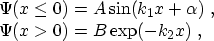
For capture processes and for emission processes where the electron faces a trapezoidal barrier, the barrier is transformed into a step function of height equal to the potential at the middle point between $x=0$ and $x=\ensuremath{x_0}$ ( $\ensuremath{{\mathcal{E}}_\mathrm{m}}$ in the left part of Fig. 3.18), $x_0$ being the position of the trap inside the dielectric. Assuming

$$\begin{array}{l} \Psi(x\le 0) = A \sin(k_1 x + \alpha)\ ,\\ \Psi(x>0) = B\exp(-k_2 x)\ , \end{array}$$ (3.136)

the wave function at the position of the trap becomes

$$\Psi(x) = A \sin \left( \arctan \left( \frac{\ensuremath{m_\mathr... ...}{\ensuremath{m_\mathrm{eff}}}\frac{k_1}{k_2 } \right) \right) \exp (-k_2 x)\ ,$$ (3.137)

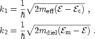
where $m_\mathrm{diel}$ and $m_\mathrm{eff}$ are the electron masses in the dielectric and the neighboring electrode, respectively. The wave numbers are given by

$$\renewedcommand{arraystretch}{2.0}\begin{array}{l} \displaystyle ... ...hrm{diel}}(\ensuremath{{\mathcal{E}}_\mathrm{m}}-{\mathcal{E}})}\ . \end{array}$$ (3.138)

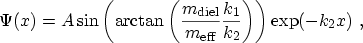
For emission processes in which the barrier is triangular (the electron energy is above the dielectric conduction band at some point between the trap and the anode), two regions in the dielectric must be distinguished. The first one, between the interface at $x=0$ and the point $x=\ensuremath{x_\mathrm{FN}}$ (see the right part of Fig. 3.18) has the height $\ensuremath{{\mathcal{E}}_\mathrm{FN}}$. The height of the approximated barrier in the other region is then the value of the barrier, $\ensuremath{{\mathcal{E}}_\mathrm{m}}$, in the middle point between $x=\ensuremath{x_\mathrm{FN}}$ and the position of the trap $x=\ensuremath{x_0}$. With this new barrier and the assumptions for the wave functions in the three regions

$$\Psi(x \le 0) = A \sin (k_1 x + \alpha_1)\ ,$$ (3.139)

$$\Psi(0 < x \le \ensuremath{x_\mathrm{FN}}) = B \sin (k_2 x + \alpha_2)\ ,$$ (3.140)

$$\Psi(\ensuremath{x_\mathrm{FN}}< x \le \ensuremath{x_0}) = C \exp(-k_3 (x-\ensuremath{x_\mathrm{FN}})) \ ,$$ (3.141)

the wave function at the position of the trap becomes

$$\Psi (x)=A\frac{\sin \alpha_1 }{\sin \alpha_2} \sin \left( k_2 \e... ...}}+ \alpha_2 \right) \exp \left( -k_3(x - \ensuremath{x_\mathrm{FN}})\right)\ ,$$ (3.142)

with the symbols

$$\renewedcommand{arraystretch}{2.0}\begin{array}{l} \displaystyle ... ...an \left( \frac{k_2}{k_3}\right) -k_2 \ensuremath{x_\mathrm{FN}}\ . \end{array}$$ (3.143)

The corresponding wave numbers are given as

$$\renewedcommand{arraystretch}{2.0}\begin{array}{l} \displaystyle ... ...hrm{diel}}(\ensuremath{{\mathcal{E}}_\mathrm{m}}-{\mathcal{E}})}\ . \end{array}$$ (3.144)

Using expression (3.137) and (3.142), the integration in (3.134) can be performed analytically which allows the capture and emission probabilities to be calculated without the need for numerical integration.

A. Gehring: Simulation of Tunneling in Semiconductor Devices