4.2 The Tunneling Model
The main problem for the integration of tunneling current models in a device
simulator such as MINIMOS-NT is that tunneling is a non-local effect. In contrast
to the current density described by the drift-diffusion (2.4) or
energy-transport model (2.8), the current density at a certain point does
not only depend on quantities at the same point, but on geometrical properties
such as the thickness of the segment considered for tunneling. Thus, the
tunneling current contribution cannot be simply derived from local quantities
alone. In MINIMOS-NT the tunneling current is calculated between two boundaries
of insulator or semiconductor segments. The boundaries are either specified
by the user (see Appendix D) or found automatically. In the
latter case the tunneling boundaries are identified as the first two
boundaries of the specified segment to neighboring non-insulating materials
which have the smallest distance4.1. For each grid node at the specified boundary, the node on the
other boundary with minimum distance is selected as partner node. It may
happen that some nodes share their partner nodes, such as the nodes  , and
, and
 in Fig. 4.1. Thus, this implementation is valid for
non-orthogonal grids, too.
in Fig. 4.1. Thus, this implementation is valid for
non-orthogonal grids, too.
Figure 4.1:
Boundary node - partner node pairs. The considered
boundaries are indicated by bold lines.
|
|
The physical quantities at the neighboring segments, such as the carrier
concentration, the electrostatic potential, and the carrier temperature, are
passed to the tunneling model which is evaluated for each boundary grid
point. Then, the tunneling current density is calculated by one of the models
described in Section 3 and the total tunneling current is found by
summation of the current density along the boundary and multiplication with
the area of the grid element. A projection factor  is calculated for
every node to account for pair nodes which do not lie directly opposite to
each other:
is calculated for
every node to account for pair nodes which do not lie directly opposite to
each other:
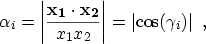 |
(4.1) |
where
 points from the boundary node to the partner node and
 to the next node on the boundary. In Fig. 4.1, for
example, the tunneling current is calculated for the boundary nodes and
with respect to the partner node
to the next node on the boundary. In Fig. 4.1, for
example, the tunneling current is calculated for the boundary nodes and
with respect to the partner node  .
.
The total tunneling current is calculated by a summation along the boundary
with length  which consists of
  segments
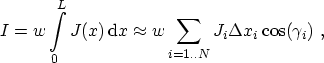 |
(4.2) |
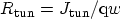
where  is the gate
width,
is the gate
width,  the local tunneling current density, and
 the
interface length associated with the node . The local tunneling current
density is added self-consistently to the continuity equation of the
neighboring segments by means of an additional recombination term
the
interface length associated with the node . The local tunneling current
density is added self-consistently to the continuity equation of the
neighboring segments by means of an additional recombination term
 |
(4.3) |
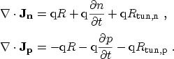
In MINIMOS-NT the NEWTON4.2 method is used to calculate the
solution vector consisting of  ,
,  , and
, and  at step
  from the
matrix equation
from the
matrix equation
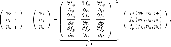 |
(4.4) |
where  ,
,  , and
, and  denote the control equations determining the
electrostatic potential, the electron concentration, and the hole
concentration. Since
denote the control equations determining the
electrostatic potential, the electron concentration, and the hole
concentration. Since
 modifies all solution variables, the JACOBI
an4.3
modifies all solution variables, the JACOBI
an4.3
 must be modified to achieve better convergence of the
NEWTON solver. Therefore, the derivatives of the additional recombination
term with respect to the potential, electron concentration, and hole
concentration
must be modified to achieve better convergence of the
NEWTON solver. Therefore, the derivatives of the additional recombination
term with respect to the potential, electron concentration, and hole
concentration
have to be calculated. For the FOWLER-NORDHEIM, SCHUEGRAF, and
FRENKEL-POOLE model, the derivatives are calculated analytically while for
all other models they are calculated numerically.
Subsections
A. Gehring: Simulation of Tunneling in Semiconductor Devices
![\includegraphics[width=.8\linewidth]{figures/mmntGrid}](img703.png)