can be formulated as
Charge trapping models found in literature usually assume elastic electron tunneling, which ignores the atomic configuration of the defects. In the Franck-Condon theory [107, 108, 109, 110], however, changes in the defect configuration play a crucial role in the charge trapping process. For instance, this theory predicts that the defect levels can be subject to a shift [111, 112, 113, 114] (discussed in Section 2.2). In order to support the physical understanding of such trapping processes, one has to deal with the basics of microscopic theories, which provide the most complete description of a physical process, such as charge trapping.
Therefore, the Schrödinger equation [92, 91] for a system involving electrons and
nuclei is taken as a starting point. Its Hamiltonian can be formulated as
 and
and  refer to nuclei and electrons, respectively.
  and
and
 are the coordinates of a certain electron
  or a certain nucleus
  ,
respectively, whereas the curly braces stand for the whole set of coordinates,
such as
,
respectively, whereas the curly braces stand for the whole set of coordinates,
such as  ,
,  ,
,  ,
,  for
for  . The Hamiltonian
  contains all
contributions from the electrons (
contains all
contributions from the electrons ( ) and nuclei (
 ) kinetic energies as well
as from the Coulombic electron-electron
) kinetic energies as well
as from the Coulombic electron-electron  , nucleus-nucleus
  , and
electron-nucleus
, and
electron-nucleus  interactions. Then, the Schrödinger equation reads
where the energy of the whole system of the electrons and the nuclei is denoted as
interactions. Then, the Schrödinger equation reads
where the energy of the whole system of the electrons and the nuclei is denoted as
 . It is important to note at this point that the wavefunctions
  depend on all positions of the electrons as well as the nuclei and thus the equation
(2.14) cannot be solved due to its mathematical complexity.
depend on all positions of the electrons as well as the nuclei and thus the equation
(2.14) cannot be solved due to its mathematical complexity.
In order to obtain an approximate solution, one usually employs the Born-Oppenheimer
approximation, also known as the adiabatic approximation [92, 91], which states
that the electrons move much faster than the nuclei. In this picture, the electrons
instantaneously adapt to each atomic configuration and the motion of the nuclei can
be neglected for the solution of the electron system. Based on this assumption the
wavefunction  can be split into an electron (
 ) and a
nuclei (
) and a
nuclei ( ) part.

 .
.  stands for the many-electron wavefunction, which is a function of
the electron coordinates
stands for the many-electron wavefunction, which is a function of
the electron coordinates  . The nuclei have fixed positions
  and enter the
equation (2.16) as parameters only. Consequently, their positive charges form an
external potential
and enter the
equation (2.16) as parameters only. Consequently, their positive charges form an
external potential  to the electron system. The eigenvalues
 of equation (2.16) re-enter the Schrödinger equation of the nuclei system,
and act as an external potential, in which the nuclei move. This potential is therefore
referred to as the adiabatic potential or the potential energy surface. The nuclei in
the Schrödinger equation (2.17) are treated as quantum mechanical particles.
Therefore, they cannot be visualized as being to be located at certain points in space
but are described by their wavefunctions
of equation (2.16) re-enter the Schrödinger equation of the nuclei system,
and act as an external potential, in which the nuclei move. This potential is therefore
referred to as the adiabatic potential or the potential energy surface. The nuclei in
the Schrödinger equation (2.17) are treated as quantum mechanical particles.
Therefore, they cannot be visualized as being to be located at certain points in space
but are described by their wavefunctions  . Furthermore, the energy
spectrum of the nuclei system is quantized and includes discretized excitations known
as lattice vibrations in crystals. In quantum chemistry, the nuclei system is frequently
visualized in so-called configuration coordinate diagrams (see Fig. 2.2). The
ordinate of these diagrams represents the total energy
. Furthermore, the energy
spectrum of the nuclei system is quantized and includes discretized excitations known
as lattice vibrations in crystals. In quantum chemistry, the nuclei system is frequently
visualized in so-called configuration coordinate diagrams (see Fig. 2.2). The
ordinate of these diagrams represents the total energy  presuming that
the electron system is in its ground state. The abscissa is the configuration
coordinate
presuming that
the electron system is in its ground state. The abscissa is the configuration
coordinate  , which summarizes the nuclei configuration
  in one
quantity. It is important to note here that the coupling of the two Schrödinger
equations (2.16) and (2.17) results in so-called ‘vibronic’ states, which are
combinations of the electronic and the vibrational states and are defined by the
wavefunctions
in one
quantity. It is important to note here that the coupling of the two Schrödinger
equations (2.16) and (2.17) results in so-called ‘vibronic’ states, which are
combinations of the electronic and the vibrational states and are defined by the
wavefunctions  and their corresponding energy
 .
.
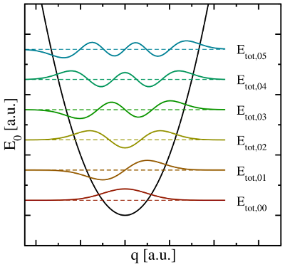
 , where the electron system is assumed to be in its ground state.
The abscissa is the configuration coordinate
, where the electron system is assumed to be in its ground state.
The abscissa is the configuration coordinate  , which describes the atomic
configuration
, which describes the atomic
configuration  . The quantum mechanical nature of the nuclei is reflected
in the formation of wavefunctions
. The quantum mechanical nature of the nuclei is reflected
in the formation of wavefunctions  (colored lines), each of which has
its corresponding discrete energies
(colored lines), each of which has
its corresponding discrete energies  .
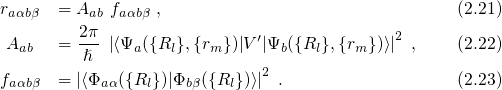
.According to the Franck-Condon principle [107, 108, 109, 110], these vibronic transitions involve a change in the electronic as well as in the vibrational state. The corresponding rate can be calculated using Fermi’s golden rule (see Appendix A.1)
with being the perturbation operator.
  and
and  denote the initial and the
final vibronic state, respectively, where the latin and greek symbols refer
to the electronic and vibrational states. According to the Franck-Condon
approximation, the matrix element
denote the initial and the
final vibronic state, respectively, where the latin and greek symbols refer
to the electronic and vibrational states. According to the Franck-Condon
approximation, the matrix element  can be separated into two factors:

 denotes the electronic matrix element and is associated with an
electronic transition, for instance electron or hole tunneling in the case of charge
trapping in defects. The Franck-Condon factor
denotes the electronic matrix element and is associated with an
electronic transition, for instance electron or hole tunneling in the case of charge
trapping in defects. The Franck-Condon factor  gives the probability of
the vibrational transition, which is determined by the overlap of the nuclei
wavefunctions. The probability for such a transition is lower than that for the
electron transition. Therefore,
gives the probability of
the vibrational transition, which is determined by the overlap of the nuclei
wavefunctions. The probability for such a transition is lower than that for the
electron transition. Therefore,  becomes the decisive factor in equation
(2.21).
becomes the decisive factor in equation
(2.21).