3.3 Box Integration Method

To overcome the limitations of the finite difference method the box integration method [49, p.191] [50]^3.1 can be used. The simulation domain is partitioned into subdomains without overlap or exclusion. An example can be seen in Fig. 3.3.

Figure 3.3: A set of 13 grid points together with their associated VORONOI regions which are bounded by the dashed lines.

The subdomains are also called VORONOI^3.2 regions. A VORONOI region is defined as the set of all points that are closer to the considered grid point than to any other grid point. The differential equations are then integrated over each of the subdomains and discretized by approximating the integrals by numerical integration rules.

For an orthogonal grid structure the box integration method leads to the expressions obtained from the finite difference method.

To get a connection between the global and the local attributes of fields, a relation between the integral over a domain and the boundary of this domain must be presented. Its general form is the GREEN transformation

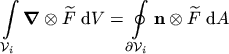$$\ensuremath{\int_{\ensuremath{\mathcal{ V }}_i} \ensuremath{\ensu... ...} \ensuremath{\otimes}\ensuremath{\widetilde{F}} \,\, \ensuremath{\mathrm{d}}A}$$ (3.16)

By reducing $\ensuremath{\widetilde{F}}$ to a vector $\ensuremath{\widetilde{F}} = \ensuremath{\boldsymbol{\mathrm{f}}}$, the theorem of GAUSS is obtained

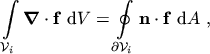$$\ensuremath{\int_{\ensuremath{\mathcal{ V }}_i} \ensuremath{\ensu... ...th{\cdot}\ensuremath{\boldsymbol{\mathrm{f}}} \,\, \ensuremath{\mathrm{d}}A}\ ,$$ (3.17)

where $\ensuremath{\mathcal{ V }}_i$ denotes the integration volume, $\partial \ensuremath{\mathcal{ V }}_i$ is the boundary of the volume and $\ensuremath{\boldsymbol{\mathrm{n}}}$ is the unity vector which is normal to the boundary and points from the inside to the outside.

Subsections

• 3.3.1 POISSON's Equation
• 3.3.2 Six Moments Transport Model
  • 3.3.2.1 Continuity and Balance Equations
  • 3.3.2.2 Flux Equations
  • 3.3.2.3 Growth Function
  
  
• 3.3.3 Final Remarks

M. Gritsch: Numerical Modeling of Silicon-on-Insulator MOSFETs PDF