7.4 Performance Analysis

The trend of increasing clock speeds has led to the problem that CPUs require data at a faster rate than memories are able to supply it.

From a software point of view, the currently available calculation resources of computer systems require the utilization of various paradigms such as object-orientation programming, generic programming, functional programming, and meta-programming, as introduced in Section 4.2, to obtain an overall high performance. The most important parts of how to achieve high performance in C++ can be summarized on the one hand by static parametric polymorphism [143,94,144] for a global optimization with inlined function blocks, and on the other hand by lightweight object optimization [41] which enables allocation of simple objects to registers. This has already been demonstrated in the field of numerical analysis, yielding figures comparable to Fortran [145,100,47], the previously undisputed candidate for this kind of calculation. The C and Fortran languages do not offer techniques for a variable degree of optimization, such as controlled loop unrolling [146,143]. Such tasks are left to the compiler. Therefore, libraries have to use special techniques as employed by ATLAS [147] or have to rely on manually tuned code elements which have been assembled by domain experts or the vendors of the microprocessor architecture used. Thereby, a strong dependence on the vendor of the microprocessor is incurred. In short, these methods greatly complicate the development process of orthogonal high performance libraries.

To analyze the performance of the implemented GSSE approach on various computer systems, the maximum achievable performance is summarized in the following table, which shows the CPU types, the amount of RAM, and the compilers used. A balance factor (BF) is evaluated by dividing the maximum MFLOPS measured by ATLAS [147] by the maximum memory band width (MB) in megabytes per second measured with STREAM [148]. This factor states the relative cost of arithmetic calculations compared to memory access.

Type	Speed	RAM	GCC	MFLOPS	MB/s	Balance factor
P4	1 x 2.8 GHz	2 GB	4.0.3	2310.9	3045.8	0.7
AMD64	1 x 2.2 GHz	2 GB	3.4.4	3543.0	2667.7	1.2
IBMP655	8 x 1.5 GHz	64 GB	4.0.1	16361.7	4830.4	3.4
G5	4 x 2.5 GHz	8 GB	4.0.0	24434.0	3213.3	7.6
Intel Core E6600	2 x 2.4 GHz	2 GB	4.1.2	12404.0	4047.2	3.1
AMD X2 5600+	2 x 2.8 GHz	2 GB	4.1.2	17773.45	3692.2	4.8

7.4.1 GTL's Performance

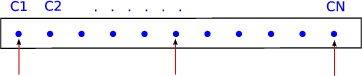
The first analysis concerns to the topological traversal for different dimensional cell complex types. First a typical representative of a 0-cell complex, e.g., an array, is traversed. The C++ STL containers, such as vector or list, are representatives and are schematically depicted in Figure 7.12, where the points represent the cells on which data values are stored.

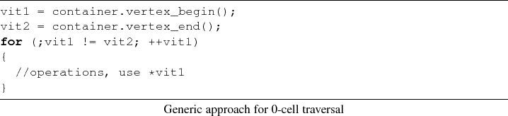
**Figure 7.12:** Topological traversal of vertices.
$\begin{figure}\begin{center}\epsfig{figure=figures/gsse_iteration_comparison_1.eps, width=8cm} \end{center} \vspace*{-0.5cm} \end{figure}$

To investigate the abstraction penalty of the generic code a simple C implementation is used without any generic overhead compared to the GTL. The next code snippet presents the C source code for a three-dimensional 0-cell complex (cube) and is followed by the generic approach:
$\begin{lstlisting}[frame=lines,label=,title={C approach for 0-cell traversal}]{}... ...(i1 = 0; i1 < sized1; i1++) { //operations, use i1, i2, i3 } \end{lstlisting}$

$\begin{lstlisting}[frame=lines,label=,title={Generic approach for 0-cell travers... ...d(); for (;vit1 != vit2; ++vit1) { //operations, use *vit1 } \end{lstlisting}$

Figures 7.13-7.16 present results obtained on four computer systems. As can be seen, the performance is comparable on different systems without incurring an abstraction penalty from the highly generic code when compared to a simple C implementation.

**Figure 7.13:** 0-cell traversal on the P4; the units are iterations per second.
$\begin{figure}\begin{center} \Large \psfrag{1e+02} [l]{$\mathrm{10}^\mathrm{2... ...al/gtl_01/performance_p4_1.ps, angle=-90, width=10cm} \end{center} \end{figure}$

**Figure 7.14:** 0-cell traversal on the AMD64 (right); the units are iterations per second.
$\begin{figure}\begin{center} \Large \psfrag{1e+02} [l]{$\mathrm{10}^\mathrm{2... ...l/gtl_01/performance_amd_1.ps, angle=-90, width=10cm} \end{center} \end{figure}$

**Figure 7.15:** 0-cell traversal on the G5; the units are iterations per second
$\begin{figure}\begin{center} \Large \psfrag{1e+02} [l]{$\mathrm{10}^\mathrm{2... ...al/gtl_01/performance_g5_1.ps, angle=-90, width=10cm} \end{center} \end{figure}$

**Figure 7.16:** 0-cell traversal on the IBM; the units are iterations per second
$\begin{figure}\begin{center} \Large \psfrag{1e+02} [l]{$\mathrm{10}^\mathrm{2... ...l/gtl_01/performance_aix_1.ps, angle=-90, width=10cm} \end{center} \end{figure}$

$\begin{figure}\begin{center} \epsfig{figure =figures/gsse_iteration_comparison_3.eps, width=5.5cm} \end{center}\vspace*{-0.5cm} \end{figure}$

Figure 7.17: Topological traversal of cells for a one-dimensional cell complex.

The source code snippets from Section 7.1.2 are used as the corresponding implementations.

**Figure 7.18:** Incidence traversal for the BGL and the GTL approach on the P4; the units are iterations per second
$\begin{figure}\begin{center} \Large \psfrag{1e+02} [l]{$\mathrm{10}^\mathrm{2... ...inal/gtl_02/performance_p4.ps, angle=-90, width=10cm} \end{center} \end{figure}$

**Figure 7.19:** Incidence traversal for the BGL and the GTL approach on the AMD64; the units are iterations per second
$\begin{figure}\begin{center} \Large \psfrag{1e+02} [l]{$\mathrm{10}^\mathrm{2... ...nal/gtl_02/performance_amd.ps, angle=-90, width=10cm} \end{center} \end{figure}$

**Figure 7.20:** Incidence traversal for the BGL and the GTL approach on the G5; the units are iterations per second
$\begin{figure}\begin{center} \Large \psfrag{1e+02} [l]{$\mathrm{10}^\mathrm{2... ...inal/gtl_02/performance_g5.ps, angle=-90, width=10cm} \end{center} \end{figure}$

**Figure 7.21:** Incidence traversal for the BGL and the GTL approach on the IBM; the units are iterations per second
$\begin{figure}\begin{center} \Large \psfrag{1e+02} [l]{$\mathrm{10}^\mathrm{2... ...nal/gtl_02/performance_ibm.ps, angle=-90, width=10cm} \end{center} \end{figure}$

7.4.2 GFL's Performance

The second analysis is related to the analysis of the abstraction penalty of the generic functor library. Due to the use of meta-programming and its evaluation at compile-time, the calculation associated with the specified equations can be highly optimized for the whole application by the compiler [149]. As a base foundation the Blitz++ benchmark system is used which uses a vector operation (DAXPY) $f = \alpha \cdot x + y$ , evaluated with different vector sizes for

. The influence on different machines can be clearly separated into the system-related differences and the compiler-based differences. Therefore, the first benchmarks are related to different compiler versions of the GCC. Next, a comparison of all machines is given.

For a rigorous analysis, different implementations in C++ are analyzed and compared to a hand-optimized Fortran 77 implementation on different computer architectures:

**Figure 7.22:** Evolution of compiler enhancements on the P4 for the DAXPY benchmark using the GCC 4.0.4
$\begin{figure}\begin{center} \Large \psfrag{1e+02} [l]{$\mathrm{10}^\mathrm{2... ...p4_2_in13.iue.tuwien.ac.at.ps, angle=-90, width=10cm} \end{center} \end{figure}$

**Figure 7.23:** Evolution of compiler enhancements on the P4 for the DAXPY benchmark using the GCC 4.1.2
$\begin{figure}\begin{center} \Large \psfrag{1e+02} [l]{$\mathrm{10}^\mathrm{2... ...p4_2_in13.iue.tuwien.ac.at.ps, angle=-90, width=10cm} \end{center} \end{figure}$

**Figure 7.24:** Evolution of compiler enhancements on the P4 for the DAXPY benchmark using the GCC 4.2.1
$\begin{figure}\begin{center} \Large \psfrag{1e+02} [l]{$\mathrm{10}^\mathrm{2... ...p4_2_in13.iue.tuwien.ac.at.ps, angle=-90, width=10cm} \end{center} \end{figure}$

**Figure 7.25:** Evolution of compiler enhancements on the AMD X2 for the DAXPY benchmark using the GCC 4.0.4
$\begin{figure}\begin{center} \Large \psfrag{1e+02} [l]{$\mathrm{10}^\mathrm{2... ...formance_gcc404_amd_1_in13.ps, angle=-90, width=10cm} \end{center} \end{figure}$

**Figure 7.26:** Evolution of compiler enhancements on the AMD X2 for the DAXPY benchmark using the GCC 4.1.2
$\begin{figure}\begin{center} \Large \psfrag{1e+02} [l]{$\mathrm{10}^\mathrm{2... ...formance_gcc412_amd_6_in13.ps, angle=-90, width=10cm} \end{center} \end{figure}$

**Figure 7.27:** Evolution of compiler enhancements on the AMD X2 for the DAXPY benchmark using the GCC 4.2.1
$\begin{figure}\begin{center} \Large \psfrag{1e+02} [l]{$\mathrm{10}^\mathrm{2... ...formance_gcc412_amd_6_in13.ps, angle=-90, width=10cm} \end{center} \end{figure}$

As can be seen, the GSSE performs well with recent compilers such as the GCC 4.2.1 compiler generation. Another important point can be seen. The overall computer performance has doubled within the last two years.

To analyze the dependence on the machine in more detail, the best possible compiler generation is used on all the machines and the results are provided in Figures 7.28-7.31.

**Figure 7.28:** Best compiler performance for the Intel Core using the GCC 4.2.1.
$\begin{figure}\begin{center} \Large \psfrag{1e+02} [l]{$\mathrm{10}^\mathrm{2... ...erformance_gcc421_c2_2_l08.ps, angle=-90, width=10cm} \end{center} \end{figure}$

**Figure 7.29:** Best compiler performance for the AMD X2 using the GCC 4.2.1.
$\begin{figure}\begin{center} \Large \psfrag{1e+02} [l]{$\mathrm{10}^\mathrm{2... ...e_gcc421_amd_6_single_in13.ps, angle=-90, width=10cm} \end{center} \end{figure}$

**Figure 7.30:** Best compiler performance for the G5 using the system compiler.
$\begin{figure}\begin{center} \Large \psfrag{1e+02} [l]{$\mathrm{10}^\mathrm{2... ...p4_2_in13.iue.tuwien.ac.at.ps, angle=-90, width=10cm} \end{center} \end{figure}$

**Figure 7.31:** Best compiler performance for the IBM using the system compiler.
$\begin{figure}\begin{center} \Large \psfrag{1e+02} [l]{$\mathrm{10}^\mathrm{2... ...formance_gcc_tcad_2_tcad04.ps, angle=-90, width=10cm} \end{center} \end{figure}$

Although the machine information of the Intel Core is superior to the AMD X2 system, the overall benchmarks show that the GSSE performs best on the AMD X2 with a recent compiler. A wide variety of optimization possibilities are thereby available. Recent developments and research have focused on the process of automation for this type of optimization for several architectures and compilers by the introduction of a concept called composer [151].