7.1 The Generic Topology Library

The most basic mechanisms of the GTL are the utilization of cell types and complex types, as explained theoretically in Section 1.3.2. A common topological data structure specification scheme can thereby be derived, as given in Section 5.1.

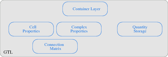
**Figure 7.2:** The generic topology library of the *GSSE*.
$\begin{figure}\begin{center} \epsfig{figure=figures/gsse2007_gtl.eps, width=12cm} \end{center}\end{figure}$

The GTL transforms each of the given theoretical concepts into a module, where the connection matrix implementation builds the base for the GTL. The poset concept and the corresponding cell topology is implemented by a cell property module, where several posets for different dimensions are stored. Also, several boundary operations for cell traversal are thereby covered. The complex module then implements the local and global cell complex properties, whereby the global cell complex uses procedurally generated incidence and adjacence information and the local cell complex requires the information stored in the connection matrix. The quantity storage module enables an interface to various container structures. Finally, the container layer uses the index space concept and implements an interface to the cell and complex properties. A topological declaration of a simplex and a cuboid object with their respective dimensions is illustrated in the next code snippet^7.1.

$\begin{lstlisting}[frame=lines,title={Cell types}]{} cell_type<0, simplex> cell_s; // vertex cell_type<3, cuboid> cell_c; // cuboid \end{lstlisting}$

The first specification describes a simple vertex element, a zero-dimensional simplex cell, whereas the second line specifies a cube, a three-dimensional cell. Based on the poset mechanism of the GTL and the concept of a boundary operator (Section 5.2 and Section 5.3), different types of incidence traversal operations are already available. This means that the complete cell topology can be used. However, the cell topology does not contain any cell complex information, such as neighboring cell information.

This information is available by the topology of cell complexes, where only a few complex types are presented in the following code snippet. It should be noted here, however that the complex type is definitely not restricted to these types of cells. Arbitrary types can be used which model the corresponding concepts.

$\begin{lstlisting}[frame=lines,title={Complex types}]{} complex_type<cell_c, loc... ...ked list / tree complex_type<cell_t, global> complex_3; // grid \end{lstlisting}$

As can be seen, a variety of data structures is thereby uniformly available. Various underlying implementations can be used with a topological formal interface, e.g., the GrAL library for the third line. Basically, the GTL represents a formal topological interface for different types of data structures. Additionally, it provides implementations for the topologies introduced in Section 5.1.

These two parts also integrate a homogeneous access to compile-time and run-time mechanisms. It is important to implement the different evaluation times separately in order to obtain an overall high performance. The following table gives an overview of the different parts of the library with their corresponding evaluation times.

	compile-time	run-time
cell topology, simplex	yes	no
cell topology, cuboid	yes	no
cell topology, polytope	no	yes
complex topology, local	no	yes
complex topology, global	yes	no

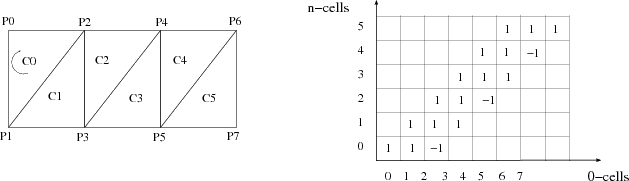
An example of the connection matrix, e.g., for a 3-simplex cell complex, is depicted in Figure 7.3:

**Figure 7.3:** Example of the connection matrix for a 3-simplex cell complex.
$\begin{figure}\centering \epsfig{figure=figures/connection_matrix.eps, width=14cm} \end{figure}$

The implementation of the container concept is given which combines the complex types (base space properties) with the data types (fiber space properties), where the indexspace property is used to introduce the distance of the data from the base space. Finally, an interface to a quantity storage is available, which is connected to the GTL by a unique identifier for each cell.

$\begin{lstlisting}[frame=lines,label=,title={Container type} ]{} typedef long data_t; container_t<complex_1, data_t ,indexspace<0> > container; \end{lstlisting}$
The given example uses an index space depth of zero, which means that the data is directly stored at the cell location.

7.1.1 The 0-Cell Complex

The best known and most widely used data structures in programming can be described by the 0-cell complex types, e.g., the data structures of the C++ STL, depicted in Figure 7.4. The reason for the common topological structure of the C++ STL data structures is the fact that the iterators cannot access any higher dimensional internal structure. One the one hand, this is one of the major advances of the iterator approach of the STL by separating data structure and algorithms. The implementation complexity is thereby significantly reduced. On the other hand, all iterators can only access the zero-dimensional cell of a data structure. Hence it is not possible, e.g., to iterate over the neighbors of a C++ std::map.

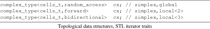
**Figure 7.4:** Representation of a 0-cell complex with a topological structure equivalent to a standard container.
$\begin{figure}\centering \epsfig{figure=figures/gsse_0cell.eps, width=8cm} \end{figure}$

The following source snippet introduces the specification of the given topological classification scheme (Section 5.1) with respect to simple well-known data structures, such as arrays or singly linked lists. The tags global and local in the following code snippet specify the locality of the complex topology.

$\begin{lstlisting}[frame=lines,label=,title={Topological data structures}]{} com... ...t / tree complex_type<cells_t, local<4> > cx; // arbitrary tree \end{lstlisting}$
These examples can also be expressed using the STL iterator traits to classify the data structures:

$\begin{lstlisting}[frame=lines,label=,title={Topological data structures, STL it... ...<2> complex_type<cells_t,bidirectional> cx; // simplex,local<3> \end{lstlisting}$

The following code snippet demonstrates the equivalence of the STL and the GTL data structures:

$\begin{lstlisting}[frame=lines,label=,title={Equivalence of data structures}]{} ... ...lent to the STL container type std::vector<data_t> container; \end{lstlisting}$
Here, the separation of the topological structure from the data specification is made explicit, in comparison to the STL, which, unfortunately, combines traversal and data access. Several problems are caused by this combined specification of a data structure^7.2. The given index-space concept is used to provide full backward compatibility for the quantity access mechanism, which means that the corresponding traversal mechanism can directly access the obtained iterator.

7.1.2 The 1-Cell Complex

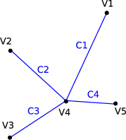
Another important representative of a commonly used cell complex is a one-dimensional complex, usually called a graph. Figure 7.5 shows a typical example. A cell of this type of cell complex is called an edge. Incidence and adjacence information exists between edges and vertices.

$\begin{figure}\centering \epsfig{figure=figures/gsse_1cellcomplex.eps, width=4cm} \end{figure}$

Figure 7.5: Representation of a 1-cell complex with cells (edges, C) and vertices (V).

In the following, the BGL facilities are compared to the traversal mechanisms provided by the GTL. The following example presents the traversal all edges of a 1-cell complex:

$\begin{lstlisting}[frame=lines,label=,title={BGL iteration}]{} typedef adjacency... ...urce1 += source(*eit, gr); test_source2 += target(*eit, gr); } \end{lstlisting}$

The GTL offers the same functionality as is demonstrated in the following code snippet. The global tag is used to demonstrate the global structure of the graph, which means that the internal data layout is prepared for dense graph storage. In terms of the BGL, an adjacency graph data structure is used.

$\begin{lstlisting}[frame=lines,label=,title={GTL's traversal}]{} typedef cell_ty... ...ovit, container); test_source2 += target(*covit, container); } \end{lstlisting}$

Related to interoperability, all algorithms developed for the BGL can be used on this structure as well, including the property map concept. The property map can be seen as a specialization of the fiber bundle approach.

7.1.3 The 2-Cell Complex

Commonly used discretization schemes use as base requirement a two-dimensional cell complex, usually called a mesh or grid. Although this cell complex can be projected onto a graph, necessary information is not available for, e.g., a finite volume or finite element method. These schemes require at least cell information, which means that a two-dimensional cell is required. A graph does not contain any cell information except the edges. In the following, the topological specification mechanism is given with respect to two important types of 2-cell complexes, a structured grid and an unstructured mesh. The storage and traversal operators of structured grids benefit greatly from the global complex topology, because all traversal operations can be rendered at compile-time. No additional cell adjacence information has to be stored compared to the unstructured mesh.

$\begin{lstlisting}[frame=lines,label=,title={Grid and mesh data types}]{} cell_t... ...rid complex_type <cellc_t, local> complex_unstructured; // mesh \end{lstlisting}$

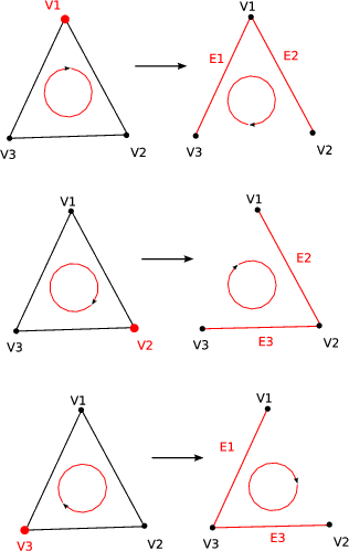
To illustrate a traversal operation offered by the GTL, the following code snippet presents a vertex-on-cell traversal with an additional incident edge traversal. A graphical representation of this traversal is given in Figure 7.6, where an arbitrary cell of the complex is used. Then a vertex-on-cell traversal is initialized, where the marked objects depict the currently evaluated objects. In the first stage of the iteration the vertex v1 is used, and the iteration is performed over the incident edge E1,E2. The iteration then continues with the remaining vertices.

$\begin{figure}\centering \epsfig{figure=figures/gsse_incidence_1.eps, width=7cm} \end{figure}$

Figure 7.6: Incidence relation and traversal operation.

The given code can be used for both of the 2-cell complex types, the complex_structured and complex_unstructured. During the loop, an edge-on-vertex traversal is created and initialized with the evaluated vertex.

$\begin{lstlisting}[frame=lines,label=,title={GTL's traversal mechanisms}]{} cell... ...(; eov_it != eove_it; ++eov_it) { //operations on edges } } \end{lstlisting}$

Traversal can be used independently of the dimension or type of cell complex. Only three topological properties have to be met by the cell complex: vertices, edges, and cells. All cell complex types which support these three objects can be used for this traversal.

To highlight the interoperability of the GTL, two examples are shown using an implementation of related work of the CGAL and GrAL. The first example presents the traversal mechanisms of the CGAL compared to the GTL. A traversal of all facets related to a cell is shown.

$\begin{lstlisting}[frame=lines,label=,title={CGAL's traversal}]{} Facet_iterator... ...(; fit != P.facets_end(); ++fit) { //operations on a facet } \end{lstlisting}$
The special geometric object Polyhedron in terms of the GTL is implemented by a common container type.

$\begin{lstlisting}[frame=lines,label=,title={GTL's traversal}]{} facet_on_cell_i... ... (; foc_it != foce_it; ++foc_it) { //operations on a facet } \end{lstlisting}$
The CGAL can be used as a complete implementation of the concepts given by the GTL. An interface layer is available to use all CGAL data types within the GTL.

The second example is related to the GrAL. The close relationship between the GrAL and the GTL makes a complete interoperability between these libraries possible. Several different grid_types can be used in GrAL, similarly to the GTL container type. The main difference is the orthogonality of the cell types and the complex types in the GTL.

$\begin{lstlisting}[frame=lines,label=,title={GrAL traversal}]{} typedef grid_typ... ...OnCellIterator cc(c); ! cc.IsDone(); ++cc) { // use cc } } \end{lstlisting}$

As can be seen, the traversal mechanisms are implemented very closely to the grid_types. The random_access property cannot be used by all traversal operations. This complicates the optimization and performance steps related to application design. The next code snippet presents the GTL implementation. It should be noted that the GTL interface can easily be implemented using the GrAL.

$\begin{lstlisting}[frame=lines,label=,title={GTL's traversal}]{} cell_iterator c... ...); for (; coc_it != coce_it; ++coc_it) { // use *coc_it } } \end{lstlisting}$
The interfaces can be exchanged easily and each of these libraries can be used with the GTL interface. Therefore the reuse of source code due to the GTL approach is a major advantage.

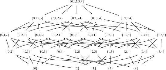
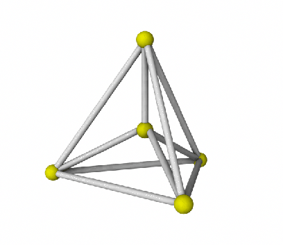
7.1.4 Higher-Dimensional Cell Complexes

The 3-cell complex is similar to the 2-cell complex, if simplex or cuboid cell types are used. Therefore the corresponding figures and code snippets are omitted. Based on the given formal definition of finite cell complexes, higher dimensions can be used as well. The theoretical mechanisms introduced in Section 1.3.2 and the implementation of the concepts given in Section 5.1 enable a clean interface for extensions, e.g., a 4-simplex, a pentachoron, depicted in Figure 7.7.

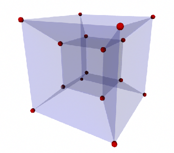
**Figure 7.7:** The cell poset of a 4-simplex as implemented by the GTL.
$\begin{figure}\centering \epsfig{figure=figures/figure19.eps, width=12.5cm}\end{figure}$

The poset of the 4-cube is omitted due to the large number of facets. Renderings of a 4-simplex and a 4-cube are presented in Figures 7.8-7.9.

**Figure 7.8:** Rendering of a 4-simplex.
$\begin{figure}\begin{center} \epsfig{figure=figures/hypersimplex.eps,width=9cm} \end{center} \end{figure}$

**Figure 7.9:** Renderings of a 4-cube.
$\begin{figure}\begin{center} \epsfig{figure=figures/cuboid_4d.eps,width=0.5\textwidth} \end{center} \end{figure}$

The following code snippet shows the implementation of an arbitrary topology with the structure of the 4-cell simplex complex. All previously presented algorithms can be used, due to the common traversal mechanisms.

$\begin{lstlisting}[frame=lines,label=,title={Four-dimensional simplex complex}]{... ...data_t; container_t<complex_t,data_t,indexspace<1> > container; \end{lstlisting}$

The GTL implements all the given data structures from Section 5.1 as well as generic algorithms for simplex and cuboid cell topologies of arbitrary dimensions.

7.1.5 Data Access

Separated by the fiber bundle approach, the stored data corresponding to the topological elements, such as vertices or edges, is available orthogonally by an element identifier, e.g., element number. During initialization, the quantity accessor q is bound to a specific domain with its quantity key. To access the underlying data, the operator() is evaluated with a vertex of the cell complex as argument and returns a reference to the stored value.

$\begin{lstlisting}[frame=lines,label=,title={Quantity assignment}] string key_qu... ... quan_t q = scalar_quan(domain, key_quan); quan(vertex) = 1.0; \end{lstlisting}$

The implementation of the fiber bundle approach in the GTL follows:
$\begin{lstlisting}[frame=lines,title={Data accessors for the container}]{} value... ...key); value = container.get_value(*vertex_on_cell , quan_key ); \end{lstlisting}$
As can be seen, the base_index selects the respective fiber, whereas the quan_key selects the corresponding fiber element. In contrast to the cursor and property map concept, the fiber bundle approach allows traversal operations within fiber space as well:
$\begin{lstlisting}[frame=lines,title={Fiber access}]{} fiber = container.get_fib... ...dex); for (it = fiber.begin(); it != fiber.end(); ++it) // ... \end{lstlisting}$
It is also possible to extract a section, which means that a whole data set attached to a base space can be returned:

$\begin{lstlisting}[frame=lines,title={Section access}]{} f_section = container.g... ...or (it = f_section.begin(); it != f_section.end(); ++it) // .. \end{lstlisting}$