12.2 Overview of Topography Simulation

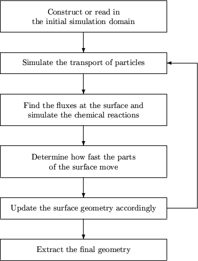
Figure 12.1: Overview of the general simulation flow of topography simulations.

Before immersing into the details of the simulation, a typical CVD (chemical vapor deposition) process is discussed [111]. The chemical reaction can happen in the gas phase, where it is called a homogeneous reaction, or at the boundary between gas and wafer, where it is called a heterogeneous reaction. Homogeneous reactions are not desired in CVD processes since they lead to the formation of clusters and thus to defects in the film. The heterogeneous reactions, however, yield high quality films and run selectively in areas where the temperature is high enough. During heterogeneous reactions the surface of the substrate often acts as a catalyst. Concerning CVD processes, the following chemical reactions are discerned: pyrolysis (heterogeneous decomposition reaction), reduction, oxidation, and hydrolysis.

The whole deposition or etching process, including the reactor scale processes which were not considered, can be divided into several parts.

• Transport of the reactants by convection through the reactor to the deposition region. The reactants are solved in carrier gas. This step is governed by the Navier-Stokes equation.
• Transport of the reactants from the convective zone through the boundary layer to the wafer surface.
• Adsorption of the reactants at the wafer surface.
• Surface reaction: dissociation of the molecules, surface diffusion of the radicals, incorporation of the radicals in the solid structure, and formation of byproducts.
• Desorption of the byproducts.
• Transport of the byproducts from the wafer surface through the boundary layer to the convective zone.
• Transport of the byproducts by convection away from the features.

Here the boundary layer is the small region above the wafer surface where the velocity of the flow of the gas is between zero at the surface and the velocity of the flow in the convective zone. Operating the equipment the temperature, the pressure and the amount of species entering the reactor can be adjusted. These three parameters influence the transport near the wafer surface and the surface deposition reactions which are discussed in two of the following sections.

The feature scale simulation of deposition and etching processes can be divided into three main steps. The according simulation flow of a typical topography simulation is shown in Figure 12.1.

• The transport of particles in the boundary layer above the wafer must be simulated. It can happen in the radiosity or diffusion regime (cf. Section 12.3).
• The fluxes of particles at the wafer surface found in the previous step determine the chemical reactions that take place at the wafer surface (cf. Sections 12.5 and 12.6).
• The surface of the wafer changes according to the previous steps. Describing the wafer surface and its change due to the fluxes of etchants and particles to be deposited is an important part of topography simulations and will be discussed in detail in Chapter 13.

The rest of this chapter and Chapter 13 are devoted to the simulation of these main steps. Before we go into details, we recall some chemical facts.

The coupling between gas concentrations $c_i$ within the reactor space and the fluxes $\Gamma_i$ towards the surface is given by the relation

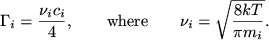$$\Gamma_i = {\nu_i c_i\over4}, \qquad\textrm{where}\qquad \nu_i = \sqrt{\frac{8 k T}{\pi m_i}}.$$ (12.1)

Here $\nu_i$ is the average molecular velocity of gas species $i$ with a molar mass $m_i$.

Relating pressure, volume, and temperature, the state equation of the ideal gas is

$$P V = n R_0 T,$$

where $P$ denotes pressure, $V$ volume, $n$ the number of moles, $R_0=8.31447\,\mathrm{J / (mol \cdot K)}$ the universal gas constant and $T$ absolute temperature. Using $n=N/N_A$, where $N$ is the number of molecules and $N_A$ the Avogadro constant, and introducing the Boltzmann constant $k$ as $k:=R_0/N_A$, the state equation can also be written as

$$P V = N k T,$$

where $k=1.38065\cdot{10}^{-23}\,\mathrm{J/K}$. In the form

$$P = k C T$$ (12.2)

the state equation relates pressure, temperature, and concentration. As the unit of pressure, $\mathrm{Torr}$ is usually used by equipment manufacturers. In SI units this is $1\,\mathrm{Torr} = 133.322\,\mathrm{Pa}$.

The classic Langmuir adsorption model [111] describes how gas adsorption on a solid surface depends on pressure via the equation $C_i=saf/(1+af)$, where $C_i$ is the concentration of adsorbed gas molecules, $a$ a constant, $f$ the gas fugacity, and $s$ the concentration of potential adsorption sites on the surface.