2.3.2 Odd Moments: Mobilities

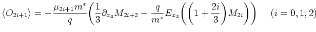
As the odd equilibrium values vanish, the macroscopic relaxation time approximation simplifies. To approximate the odd scattering terms we introduce the mobilities [GJK⁺04] in the odd equations. By setting

$$\tau \hat{=} \frac{m^* \mu}{q}$$ (2.56)

we get a formal correspondence between relaxation times and mobilities for parabolic bands. If $\mu$ and $q$ have the same sign, then $\tau$ is positive.

With this correspondence we get:

$$\langle O_{2i+1}\rangle = - \frac{\mu_{2i+1} m^{*}}{q} \bigg( \fr... ...3} \bigg( \bigg(1 + \frac{2i}{3}\bigg)M_{2i}\bigg) \bigg) \quad (i=0,1,2)$$ (2.57)

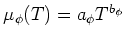One possibility to model $\mu$ is as a function depending on the the local temperature $T_n(x)$. Hence the equations depend in a nonlinear way on $M_2$ and $M_0$. Information about the scattering term can be encoded into a fitting ansatz for the mobilities, for example in the form $\mu_{\phi} (T) = a_{\phi} T^{b_{\phi}}$ with fitting parameters $a_{\phi},b_{\phi}$.

Alternatively, we can approximate the mobilities as functions of temperature and doping using results from bulk Monte Carlo simulations, see Section 2.3.4.