![dM-- -λ--
dt = - γ [M × Heff ] - γ MS [M × [M × Heff ]].](dissertation51x.png)
In 1932, Bloch reported the first description of the time-dependent motion of uncoupled and undamped magnetic moments [136]. In 1935, Landau and Lifshitz [141] have proposed an equation describing the damped motion of the magnetization in a ferromagnet, known as the Landau-Lifshitz (LL) equation [17]:
|
| (5.1) |
Here, M is the magnetization, MS is the saturation magnetization (M ⋅M = MS2), H eff is the effective magnetic field, λ is a phenomenological damping parameter, γ = g|e|∕2me is the gyromagnetic ratio, where g is the g-factor (g=2 for free electrons), e and me are the electron charge and mass, respectively.
The first term -γ![[M × Heff]](dissertation52x.png) in Equation 5.1 describes the magnetization precession around the effective
magnetic field. This form of magnetic precession is easily obtained from the classical mechanical equation
[136]
in Equation 5.1 describes the magnetization precession around the effective
magnetic field. This form of magnetic precession is easily obtained from the classical mechanical equation
[136]
 | (5.2) |
which describes the rotation of a rigid body. Here, P is the angular momentum and L is the torque acting on the body.
Then, using the magneto-mechanical ratio J = γP and substituting the magnetic torque L = ![[J × Heff ]](dissertation54x.png) Equation 5.2
obtains the form:
Equation 5.2
obtains the form:
![dJ- = - γ [J × Heff ].
dt](dissertation55x.png) | (5.3) |
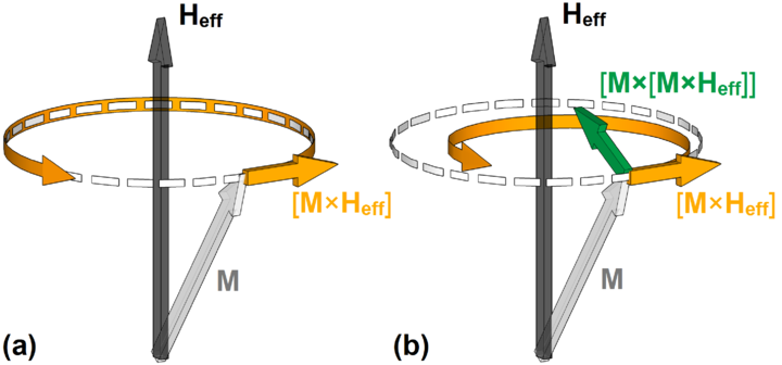
By dividing Equation 5.3 by magnetic constant μ0 the equation is converted to the version of the Landau-Lifshitz equation for undamped rotation of the magnetization (Figure 5.1a):
![dM
---- = - γ [M × Heff ].
dt](dissertation56x.png) | (5.4) |
The second term in Equation 5.1 with the double vector product -
![[M × [M × Heff ]]](dissertation58x.png) was chosen based on purely
phenomenological reasons that can be described as follows: (i) the damping process should lead the magnetization to the
state with minimum energy (parallel to the effective field); (ii) the magnetization magnitude M should remain constant
(Figure 5.1b).
was chosen based on purely
phenomenological reasons that can be described as follows: (i) the damping process should lead the magnetization to the
state with minimum energy (parallel to the effective field); (ii) the magnetization magnitude M should remain constant
(Figure 5.1b).
The Equation 5.1 could be used only in a case of small damping. In 1955, Gilbert proposed the equation which describes the strong damping in the thin films [77]:
![dM [ [ α dM ]]
---- = - γ M × Heff - --------- .
dt γMS dt](dissertation60x.png) | (5.5) |
Here, α is the Gilbert damping parameter. The Equation 5.5 is inconvenient to use, because it involves the time derivative of the magnetization dM∕dt on both sides. By using algebraic manipulations, Equation 5.5 can be easily transformed into an explicit form
![dM-- = - ---γ---- [M × H ] - ---γ-----α--[M × [M × H ]],
dt (1 + α2) eff (1 + α2 )MS eff](dissertation61x.png) | (5.6) |
which gives us the Landau-Lifshitz-Gilbert (LLG) equation. LLG equation has the form of the LL equation if the
gyromagnetic ratio γ in LL is replaced by γ∕ and admit α = λ. To get more numerically tractable version of the
Equation 5.6, it is usually divided by MS:
and admit α = λ. To get more numerically tractable version of the
Equation 5.6, it is usually divided by MS:
![dm γ γ
----= - ------2-[m × Heff] - ------2-α [m × [m × Heff]].
dt (1 + α ) (1 + α )](dissertation63x.png) | (5.7) |
Here, m = M∕MS is the normalized vector of the magnetization.
The LLG Equation 5.7 describes the MRAM switching by magnetic field. In order to be able to describe a switching in STT-MRAM, Equation 5.5 must be supplemented by an additional spin transfer torque term τ as follows [247],[267]:
![[ ]
dm--= - γ [m × Heff ] + α m × dm-- + --γ---τ,
dt dt μ0MS](dissertation64x.png) | (5.8) |
which give us a more general version of the Landau-Lifshitz-Gilbert-Slonczewski (LLGS) equation. The Slonczewski’s spin transfer torque term τ is [265]:
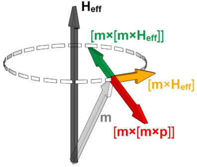
![τ = a(j)[m × [m × p]] + b(j)[m × p].](dissertation65x.png) | (5.9) |
Here, p is the normalized vector of the fixed layer magnetization, a(j) and b(j) are the current-dependent functions for the in-plane and the perpendicular torque, respectively. Unlike TMR-based structures in GMR-based structure the perpendicular torque is insignificantly small in comparison to the in-plane torque, and can be neglected [247],[267].
The numerically tractable version of LLGS Equation 5.8 is represented by [57],[105],[148]
![dm γ ℏj
dt--= - 1-+-α2-([m × Heff] + α [m × [m × Heff ]] - eM--dg(Θ )(β [m × p] - [m × [m × p]])).
S](dissertation66x.png) | (5.10) |
Here, ℏ is the reduced Planck constant, j is the current density, d is the thickness of the free layer, g(Θ) is the Slonczewski’s expression (Θ is the angle between the magnetization directions of the free and fixed layers), β is coefficient of the perpendicular torque which is usually taken to be equal α.
The LLGS Equation 5.10 is also often written in equivalent form [4],[30],[31],[64],[65], [163],[229],[248] as
![dm-- ---γ--- -g-μBj-
dt = - 1 + α2 ([m × Heff ] + α [m × [m × Heff]] + e γM d g(Θ) (β [m × p] - [m × [m × p]])).
S](dissertation67x.png) | (5.11) |
Here, g is the g-factor, μB the Bohr magneton. Equivalence of the Equation 5.10 and Equation 5.11 is easily proven by
expressing the gyromagnetic ratio for an isolated electron as γ = - .
.
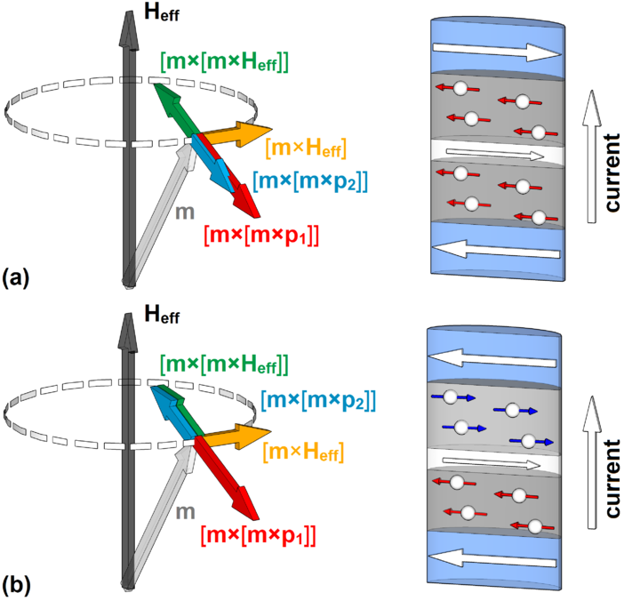
Figure 5.2 schematically illustrates the directions of the main terms of the LLGS equations. For switching the STT-MRAM the in-plane torque is the most important contribution and and the perpendicular torque is neglected in Figure 5.2.
The Slonczewski’s expression g(Θ) depends on the spacer layer material, and for a non-magnetic conducting spacer layer it is expressed by [217]
![3 3∕2 -1
g(Θ) = [- 4 + (1 + η) (3 + cos(Θ ))∕4 η ] .](dissertation70x.png) | (5.12) |
Here, η is the polarizing factor [217],[30]. For thin insulating spacer layer the Slonczewski’s expression is represented by [218]
![2 -1
g (Θ ) = 0.5 ⋅ η[1 + η ⋅ cos(Θ )] .](dissertation71x.png) | (5.13) |
The structure with the two reference layer (penta-layer structure) was investigated theoretically [167],[168] by using the Green’s function formalism combined with the free layer dynamics based on the LLG equation. A spin torque enhancement was found in the anti-parallel penta-layer (the magnetizations of the two reference layers are anti-parallel) as compared to the three-layer structure. However, this enhancement manifests itself only under dual barrier resonance tunneling conditions, when the current is high [167],[168]. At the same time, the aligned penta-layer configuration, when the magnetizations of the two reference layers are parallel to each other, was found to have a fairly low spin torque efficiency and, as a consequence, it demands high switching currents [167],[168].
An alternative way of the penta-layer structure modeling (Figure 5.3) is an extension of the LLGS Equation 5.11 by adding a second spin transfer term:
![dm γ g μBj
----= - ------2([m × Heff ]+ α [m × [m × Heff]]+------- (g1(Θ1 )(β [m × p1] - [m × [m × p1]])- g2(Θ2 )(β [m × p2] - [m × [m
dt 1 + α e γMSd](dissertation73x.png) | (5.14) |
Here, g1(Θ1) and g2(Θ2) are the Slonczewski’s expressions defined by the first and the second spacer layer, respectively. Θ1 (Θ2) is the angle between direction of the magnetization of the free and the first (second) reference layer. The minus sign before the second spin transfer torque term is introduced because the direction of spin polarized current is opposite with respect to two spacer layers. Indeed the penta-layer structure can be considered as combination of two three-layer structures with a shared free layer. Therefore, if one takes the current direction from the reference layer to the free layer as positive, then the current in the first three-layer structure and the current in the second three-layer structure flow always in opposite directions.
The effective magnetic field is the functional derivative of the magnetic energy density ε, with respect to the magnetization m [165]:
 | (5.15) |
The effective magnetic field contains the following contributions:
 | (5.16) |
Here, Hext is the external magnetic field, Hexch is the exchange field, Hani is the magnetocrystalline anisotropy field, Hdemag is the demagnetization field, Hms is the field due to magnetostatic coupling between the reference layer and the free layer, Hcurrent is the Ampere field, and Hth is the thermal field.
In magnetic materials the magnetic moments of the neighboring atoms are oriented in the same direction due to the exchange interaction. Relative deviations from the equilibrium orientations between neighboring moments causes an addition in exchange energy and are associated with non-parallel spin distributions. The expression for this energy can be written as [165]
![∫
E = A [(∇m )2] dV,
exch V](dissertation76x.png) | (5.17) |
where A is the material dependent magnetic exchange constant. The magnetic exchange field associated with this energy can be calculated as [165]
 | (5.18) |
The magnetic anisotropy is a characteristic of a ferromagnetic material which describes the fact that the properties of the magnetic material are unequal in different directions, i.e. they depend on the direction in which the measurement is made.
The anisotropy has a number of possible sources such as the properties of the crystal lattice (magnetocrystalline anisotropy), the properties of the interface between two magnetic films (interface anisotropy), and the shape of the magnetic sample (shape anisotropy). The magnetocrystalline anisotropy can manifest itself in the form of a uniaxial or a cubic anisotropy, and it is described by the corresponding description of the anisotropy energy. The interface anisotropy, that is important for description of structures with perpendicular magnetization, is usually taken into account as a kind of uniaxial anisotropy. The shape anisotropy is defined by the energy of demagnetization.
The simplest case of magnetocrystalline anisotropy is the uniaxial anisotropy. The anisotropy energy in this case can be written as [165]
 | (5.19) |
where K1 is the material anisotropy coefficient, n is the anisotropy axis. n is the easy axis, if K1 > 0 and n is normal to the easy plane, if K1 < 0.
The equation for calculating the anisotropy field [165] is
 | (5.20) |
The anisotropy energy is described by the expression [165]
![∫ [ ( ) ( )]
Eani = K1 m2xm2y + m2ym2z + m2zm2x + K2 m2xm2ym2z dV
V](dissertation80x.png) | (5.21) |
for materials with cubic anisotropy in the case when the directions of the crystal axes coincide with the directions of the coordinate axes. Here, K1 and K2 are the material anisotropy coefficient.
The cubic anisotropy field in this case is calculated as
 | (5.22) |
where D is the matrix
 | (5.23) |
In cases when the crystal axes are rotated in space relative to the coordinate axes, then mx, my, mz in Equations 5.21–5.23 should be replaced by the projection of the magnetization vector m to the corresponding axis of the crystal.
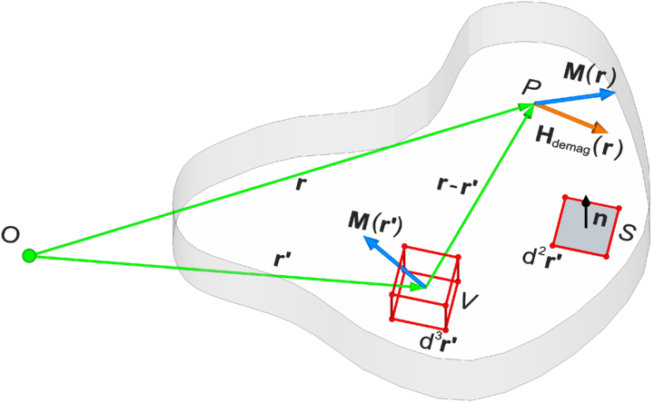
The largest contribution to the effective magnetic field is provided by the demagnetization field Hdemag. The demagnetization force is responsible for the domain structure formation in the magnetic film, unlike the above-mentioned crystalline anisotropy and exchange interaction that are responsible for unidirectional magnetization of the magnetic film. In the case of crystalline anisotropy, the preferred direction for the magnetization is along the easy axes of the crystal. In the case of exchange interaction a single-domain state with an arbitrary orientation of magnetization is preferred.
The explicit expression for Hdemag can be obtained from the Maxwell’s equations through the definition of scalar auxiliary quantities, such as surface magnetic charge σ and volume magnetic charge ρ [2],[140],[165]:
 | (5.24) |
 | (5.25) |
Using such quantities the demagnetization field Hdemag can be expressed from the scalar potential Φd of the stray field as
 | (5.26) |
where Φd(r) is expressed as
![1 [∫ ρ(r′) ∫ σ (r ′) ]
Φd (r) = ----- -----′-d3r′ + ------′d2r′ .
4πμ0 V |r - r | S |r - r|](dissertation86x.png) | (5.27) |
Next, from Equations 5.24–5.27 the equation for calculating the demagnetization field Hdemag acquires the form:
![1 [∫ (r - r′)ρ(r′) ∫ (r - r′)σ(r′) ]
Hdemag (r) = ----- --------′3---d3r′ + --------′3---d2r′ .
4πμ0 V |r - r | S |r - r |](dissertation88x.png) | (5.28) |
In an alternative way, the demagnetization field Hdemag can be obtained as a convolution of the magnetization m and a kernel representing the dipole-dipole interaction [112]:
 | (5.29) |
 | (5.30) |
Here, i,j = x,y,z are vector component.
The energy associated with the demagnetising field is given by [140]:
 | (5.31) |
Here, the demagnetization field Hdemag could be calculated based on Equation 5.28 or Equation 5.29 and the prefactor 1/2 arises from the fact that the source of Hdemag is the magnetization m itself [2].
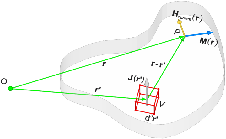
In case of the STT-MRAM, the current flowing through the free layer generates a magnetic field (Ampere’s field), which must be taken into account when calculating the effective magnetic field Heff. It is to note that this contribution does not take part in field-induced switching MRAM and must be excluded from Equation 5.16 for the effective field calculation. The Ampere field can be calculated by the Bio-Savart’s law [165]:
![∫ [ ]
-1- ′ -r---r′- 3 ′
Hcurrent = 4π J (r) × ′3 d r.
V |r - r|](dissertation92x.png) | (5.32) |
Here, J(r′) is a current density vector.
The energy associated with the Ampere field [165] is:
 | (5.33) |
The thermal fluctuations of the magnetization occur in the magnetic film when it is heated. They can be described by the introduction of an auxiliary random magnetic field. The thermal field must satisfy the following statistical properties [65],[64]:
 | (5.34) |
 | (5.35) |
where i and j are the coordinates x,y,z, the constant D measures the strength of the thermal fluctuations, and ⟨ ⟩ denotes an average taken over different realizations of the fluctuating field. The value of D is obtained from the Fokker-Planck equation [75]. According to Equations 5.34–5.35, the thermal field is uncorrelated in time and space, and Hth is described by random Gaussian distributed numbers with zero mean value.