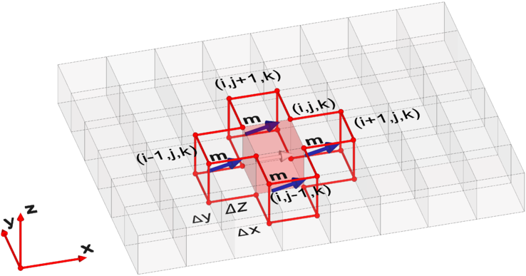
Figure 6.1: Discretization of the free layer with an elliptical cross-section.
In micromagnetics, the free layer of the pillar structure is divided by parallelepiped computational cells (Figure 6.1). Each computational cell (ΔV = ΔxΔyΔz) is represented by a unit magnetization vector m = (mx,my,mz), associated with the center of the cell. A computational cell corresponds to a uniform magnetic volume with the exchange parameter A, anisotropy constant K1 (in a case of the uniaxial anisotropy) or K1 and K2 (in a case of the cubic anisotropy), damping parameter α, saturation magnetization MS, and gyromagnetic ration γ. This parameters are the input for simulations. The dynamic of the computational cell is described by the LLG or LLGS equation, depending on the MRAM switching method.
The initial magnetization state of the free layer usually depends on the problem considered. In the simulations of the free layer switching, there are two possible initial states, defined as follows: (i) unidirectional magnetization of all cells (in the case of an ellipse, usually along the long axis); (ii) the equilibrium state, determined by the external factors and the geometry of the free layer. Depending on the initial state, important parameters such as the MRAM switching time from one magnetization state to another will vary.
There are two main approaches to calculate the effective magnetic field: field-based and energy-based approaches. In the energy-based approach, the magnetic energy is calculated directly from the discretized magnetization and the effective magnetic field is obtained from resultant energy, as a cell-averaged field [165]. The effective magnetic field in the field-based approach is calculated directly from the discretized magnetization, and the energy is obtained from the magnetic field. In the implementation the field-based approach is used: for each computational cell and each time step, the effective field is calculated by Equation 5.16, and discretized as shown below.
The external field is an input parameter for simulation and for the calculation of the effective magnetic field its value is directly added to the sum of calculated fields. The energy of a single computational cell associated with the external field can be obtained from:
 | (6.1) |
For the exchange field one must know the magnetization direction in the nearest neighbor cells (in general 6 cells). The discretized exchange field is calculated based on [165]:
 | (6.2) |
m(i′,j′,k′) denotes a magnetization in the nearest neighbor cells (Figure 6.2), and Δ is the distance between the two magnetic moments (i.e. Δx or Δy or Δz). However, according to Equation 6.2 to determine the exchange field at the boundary cell (i.e. if there is no next neighbor cell) is a problem. The most common solution to this problem is to introduce a “ghost” magnetic vector at a missing location, with a value to be the same as the nearest magnetic vector at the boundary [165].
The energy of a single computational cell associated with the exchange field can be obtained from the equation:
 | (6.3) |
When calculating the discretized anisotropy field only the magnetization direction in the cell for which the calculation is made is taken into account. For each computational cell, the anisotropy field is calculated directly on the basis of the Equation 5.20 in the case of the uniaxial anisotropy, or on the basis of Equation 5.22 in the case of the cubic anisotropy. This gives us equations for the calculation, as shown below:
in the case of of the uniaxial anisotropy:
 | (6.4) |
in the case of the cubic anisotropy:
 | (6.5) |
Here, D(i,j,k) is the space-dependent matrix, which is calculated from Equation 5.23. For both cases, the energy of a single computational cell associated with the anisotropy field can be obtained from the equation:
 | (6.6) |
The most difficult and time consuming, compared to the anisotropy field and the exchange field, is the calculation of the demagnetization field. While in the calculation of the exchange field the magnetization must be considered only in the nearest neighbor computational cells and for the calculation of the anisotropy field it is necessary to know the magnetization in a computational cell for which the calculations of the field is made, in order to calculate the demagnetization field the iteration of the magnetizations of each computational cell with the magnetization of each computational cell must be considered. Thus, the calculation of the demagnetization field occupies most of the CPU time spent for each computational time-step.
In the implementation the demagnetization field calculation based on the discretization of the Equation 5.29 is used. The resulting demagnetization field for each computational cell is calculated as the sum of the individual demagnetization contributions of the magnetization of all cells:
 | (6.7) |
Here, Nx, Ny, Nz are the grid dimensions in x, y, z direction, respectively, and G(i,j,k,i′,j′,k′) is a
space-dependent matrix of the interaction coefficients. To determine this matrix, the quantities ρ =  ,
Pu = arctan
,
Pu = arctan  , Lu = - ln
  are introduced. Pv,Pw,Lv,Lw can be obtained through permutation of
the variables u,v,w. These quantities are obtained on the basis of generalization of the equations for fast
calculations of the integrals. The derivation of the equations for fast calculations of integrals is described
in [112].
are introduced. Pv,Pw,Lv,Lw can be obtained through permutation of
the variables u,v,w. These quantities are obtained on the basis of generalization of the equations for fast
calculations of the integrals. The derivation of the equations for fast calculations of integrals is described
in [112].
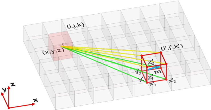
Eventually the required matrix G(i,j,k,i′,j′,k′) is obtained based on [112] (Figure 6.3):
 | (6.8) |
where
 | (6.9) |
It is to note that the matrix is symmetric, so only 6 of 9 elements of the matrix need to be calculated. Since the matrix is time-independent, it is possible to carry out the calculation only once.
The energy of a single computational cell associated with the demagnetization field can be obtained from the equation:
 | (6.10) |
The magnetostatic coupling between the reference layer and the free layer Hms(i,j,k) is calculated based on an equation similar to Equation 6.7:
 | (6.11) |
To do this, a reference magnetic layer is conditionally divided into parallelepiped elementary cells with magnetization
p =  , where Mp and MSp are the local magnetization and saturation magnetization of the reference layer,
respectively. In Equation 6.11, G(i,j,k,i′,j′,k′) is calculated based on Equation 6.8, where NPx, NPy,
NPz are the grid dimensions in x, y, z directions, and in the implementation NPx = Nx, NPy = Ny, and
NPz ≥ Nz due to the thickness of the reference layer is typically greater than the thickness of the free layer.
When the magnetization of the reference layer does not change with time, this field must be calculated only
once.
, where Mp and MSp are the local magnetization and saturation magnetization of the reference layer,
respectively. In Equation 6.11, G(i,j,k,i′,j′,k′) is calculated based on Equation 6.8, where NPx, NPy,
NPz are the grid dimensions in x, y, z directions, and in the implementation NPx = Nx, NPy = Ny, and
NPz ≥ Nz due to the thickness of the reference layer is typically greater than the thickness of the free layer.
When the magnetization of the reference layer does not change with time, this field must be calculated only
once.
The energy of a single computational cell associated with the magnetostatic coupling between the reference layer and the free layer can be obtained from the equation:
 | (6.12) |
In contrast to the demagnetization energy, one should not take the prefactor 1/2 for energy of the magnetostatic coupling between the reference layer and the free layer, since the source of the Hms in a free layer is the magnetization of the reference layer.
In the implementation the Ampere field calculation based on the discretization of the Equation 5.32 is used. Since the integrand (Equation 5.32) of the Ampere field coincides with the integrand of the volume magnetic charge in the demagnetization field calculation (Equation 5.28), the equations for fast calculations of integrals proposed in [228] are used for the demagnetization field.
The resulting Ampere field for each computational cell is calculated as the sum of the individual Ampere field contributions due to the current flowing through each cell:
![∑Nx N∑y N∑z
H (i,j,k) = -1- [J(i′,j′,k′) × G′(i,j,k, i′,j′,k′)],
current 4π ′ ′ ′
i=1 j=1k =1](dissertation117x.png) | (6.13) |
except for the cell at which this field is computed, i.e. i′≠i or j′≠j or k′≠k. In Equation 6.13, J(i′,j′,k′) is the current
density vector and G′(i,j,k,i′,j′,k′) is the space-dependent vector of the interaction coefficients. To determine this vector,
quantities ρ and Pu similar to the quantities, used for calculation of the demagnetization field (see above) are introduced,
and Lu′ =  ln
ln  . Pv, Pw, Lv′, Lw′ can be obtained through the permutation of the variables u,v,w. Eventually the
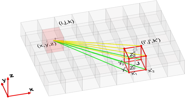
required vector G′(i,j,k,i′,j′,k′) is obtained based on [228] (Figure 6.4):
. Pv, Pw, Lv′, Lw′ can be obtained through the permutation of the variables u,v,w. Eventually the
required vector G′(i,j,k,i′,j′,k′) is obtained based on [228] (Figure 6.4):
 | (6.14) |
where
 | (6.15) |
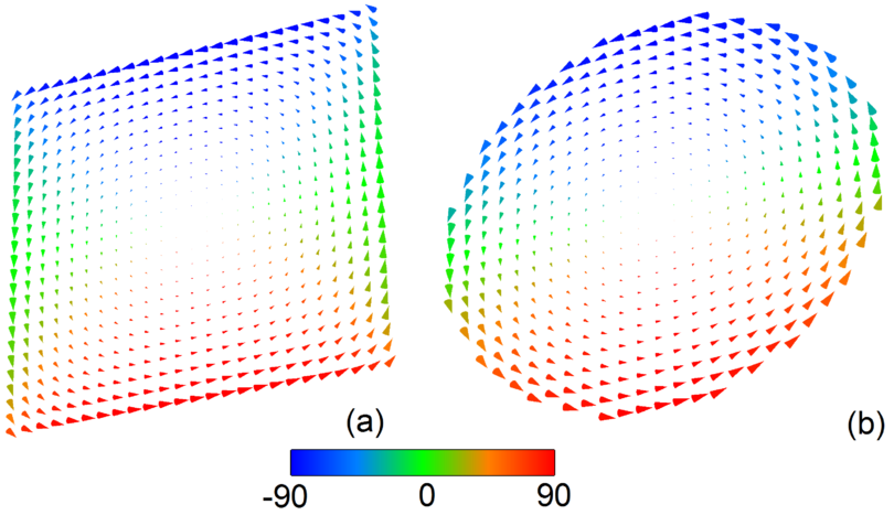
If one assumes that the current does not change with time, then the Ampere field must be calculated only once. Figure 6.5 shows an example of the Ampere field calculated for free layers with different cross-section.
The energy of a single computational cell associated with the Ampere field can be obtained from the equation:
 | (6.16) |
When calculating the discrete thermal field only the cell for which the calculation is made is taken into account [103]:
 | (6.17) |
Here, ΔV = ΔxΔyΔz is the volume of the divided cell, Δt is the time step, σ(i,j,k) = (σx,σy,σz) is a Gaussian random uncorrelated function with standard deviation equal 1.
The energy of a single computational cell associated with the thermal field can be obtained from the equation:
 | (6.18) |
The integration of LLG (LLGS) equation is done by using a fourth-order Runge-Kutta algorithm with a constant time step Δt. The new value of the magnetization at time t + Δt is derived based on the magnetization value at time t as:
 | (6.19) |
where
 | (6.20) |
 | (6.21) |
 | (6.22) |
 | (6.23) |
Here, f(m,t) is an integrable equation, i.e. LLG or LLGS.
Summarizing all described above the flowchart of the micromagnetic simulation is presented on Figure 6.6.
The full energy of a single computational cell is the sum of the corresponding contributions:
 | (6.24) |
The total energy of the free layer is the sum of full energies of every computational cell:
 | (6.25) |
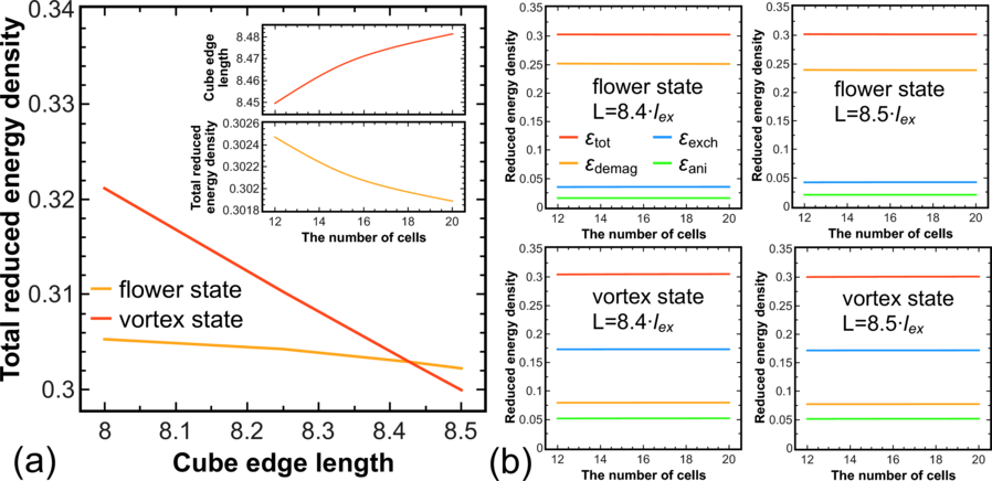
To check the correctness of the calculation of the main contributions to the total energy (demagnetization, magnetocrystalline anisotropy and exchange energy) one of the basic test problems is solved, namely, the problem of the two magnetization states of the cube [93]: “flower” and “vortex” state (Figure 6.7).

The problem is to calculate the single domain limit of a cube, i.e. the length of the cube edge where the two
magnetization states have the same total energy. The problem is material independent, so the energy density
is expressed in quantities of Km =  μ0MS2 and the length of the cube edge in l
ex =
μ0MS2 and the length of the cube edge in l
ex =  , where MS is
the saturation magnetization and A is the material exchange constant. The material anisotropy coefficient
K is taken equal to 0.1Km, and the easy axis is directed parallel to a principal axis of the cube. Different
states for the cube magnetization are obtained by calculation of the magnetization relaxation based on LLG
equation with different initial magnetization direction. For the “flower state” the initial magnetization direction
should be along the easy anisotropy axis, and for the “vortex state” it should be perpendicularly to the easy
axis.
, where MS is
the saturation magnetization and A is the material exchange constant. The material anisotropy coefficient
K is taken equal to 0.1Km, and the easy axis is directed parallel to a principal axis of the cube. Different
states for the cube magnetization are obtained by calculation of the magnetization relaxation based on LLG
equation with different initial magnetization direction. For the “flower state” the initial magnetization direction
should be along the easy anisotropy axis, and for the “vortex state” it should be perpendicularly to the easy
axis.
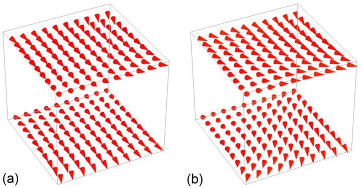
Figure 6.8a shows the simulation results for the length of cube edge from 8lex to 8.5lex, for a discretization mesh of 10 × 10 × 10. Equality of the total energy density was found for the length of cube edge equal to 8.43lex. The small bending of the curve for the total energy density for the “flower state” is determined by a transition to another kind of the “flower” with increasing the cube edge, the so called “twisted flower state”, which becomes energetically more favorable (Figure 6.9). For other discretization meshes the result is shown in inset of Figure 6.8a. Energy equality was found at about the same values of the total energy density.
Another useful check is to proof the independence of the total energy density from the discretization mesh. Figure 6.8b shows simulation results for total, demagnetization, anisotropy, and exchange energy densities for two magnetization cube states, for the edge length 8.4lex and 8.5lex. As expected, the energy density is independent on the discretization mesh from 12 × 12 × 12 to 20 × 20 × 20.