The Effective Mass Approximation

3.1 The Effective Mass Approximation

Primarily, the effective mass approximation was extensively used to describe electronic motion in the presence of slowly varying perturbations [38]. This condition for the validity of the approach is not satisfied, when the differences between the potentials in the well and barrier layers belonging to a quantum well are not small. Thus, the growing interest in quantum well structures led to a remarkable development of the effective mass theory from the regime of weak perturbations to the strong perturbation regime in microstructures [39].

In general, the energy levels and wave functions can be obtained by solving the Schrödinger equation with a proper Hamiltonian. Assuming that the many-body interactions among electrons are negligible, the motion of the electrons can be described by the one-electron Hamiltonian.

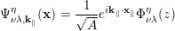
We consider electrons in the conduction band of a QCL with an electric field applied in the growth direction of the heterostructure. The total wave function can be written as the product between the periodic Bloch function at the center of the Brillouin zone and an envelope function, which is supposed to vary slowly over one period. When z is the growth direction, the free motion in the in-plane direction can be separated and the wave function in the quantum well structure is given by [40]

η -1--ik∥⋅x∥ η Ψ νλ,k∥(x) = √A e Φνλ(z)

(3.1)

where k _∥ is the in-plane wave vector, A is the cross-sectional area of the quantum well structure, and Φ_νλ^η(z) is the electron envelope function of the ν-th subband in the valley η and stage λ. Under the assumption that the periodic function is the same in all layers and due to equation (3.1) the general form of the Schrödinger equation for the quantum well structure is given by

η η η HˆΦ νλ(z) = E νλ Φνλ(z)

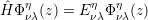(3.2)

where E_νλ^η denotes the energy and Ĥ the total Hamiltonian involving a kinetic and a potential part. Considering a junction at z₀ between the regions of two materials with dissimilar periodic potentials the current conservation is guaranteed by use of the following interface conditions [41]

( dΦη (z)) ( dΦ η(z)) Φηνλ(z)|z→z- = Φηνλ(z)|z→z+ , --1-----νλ---- |z→z -= --1------νλ---- |z→z+ 0 0 m ⋆(z ) dz 0 m ⋆(z) dz 0

(3.3)

where the upscripts ” - ” and ” + ” denote the left and right hand sides of the boundary. The condition for matching the derivative includes the effective mass m^⋆(z). Since the derivative is the momentum operator, the equation (3.3) implies the requirement that the velocity must be the same on both sides to conserve the current. The appropriate hermitian Hamiltonian can be written as

ˆ ℏ2-∂----1---∂- H = - 2 ∂zm ⋆(z)∂z + V (z).

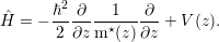(3.4)

It is of Sturm-Liouville form, which implies that the eigenvalues are real and the eigenfunctions corresponding to different eigenvalues are orthogonal [42]. The potential applied to the Schrödinger equation takes the form

V (z) = V0 (z)- eF z - eφ(z).

(3.5)

Here, V₀ is the conduction band edge, e is the elementary charge, F denotes the external electric field, and φ is the electrostatic potential.

A derivation of the effective mass equation based on the main assumption that the envelope functions are slowly varying on the scale of the lattice period, is provided in Appendix A. In this context, it should be mentioned that there is no possibility of a rigorous derivation. It is about heuristic arguments, which is generally a common practice in quantum mechanics. Nevertheless, for pedagogical purposes it is interesting to gain insight into these details.

[next] [front] [up]