The electronic subbands of the conduction band near the zone center of the Brillouin zone and the corresponding envelope functions are determined by solving the Schrödinger equation selfconsistently with the Poisson equation. Poisson’s equation plays a fundamental role in semiconductor device modeling. It is one of the basic equations in electrostatics and can be derived from the Maxwell equation
|
| (3.6) |
and the material relation
 | (3.7) |
Due to the translational symmetry of QCL structures, the electrostatic potential φ has the same profile in each stage. With F = -∇φ it satisfies the Poisson equation [43]
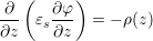 | (3.8) |
where εs denotes the static dielectric permittivity which is assumed to have an effective constant value within a material segment. The space charge density ρ in stage λ is determined from the carrier and doping concentrations, n(z) and ND+(z).
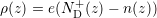 | (3.9) |
The carrier concentration is related to the wave functions by
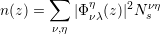 | (3.10) |
where the sum is over the subbands and the valleys, respectively. Nsνη is the electron sheet density according to [44]
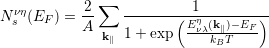 | (3.11) |
where the Fermi-Dirac distribution is used for the in-plane electron distribution in each subband, and assuming charge conservation in each stage, a position independent quasi Fermi level EF can be defined [45]. The presented scheme for the Schrödinger-Poisson solver considers a subproblem not coupled to the transport equation [46]. In the parabolic band approximation the electronic dispersion relation Eνλ η (k∥) is given by
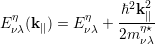 | (3.12) |
By means of the ”sum-to-integral” rule [47]
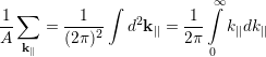 | (3.13) |
and the intergral identity
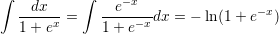 | (3.14) |
the electron sheet density reads
![kBT m η⋆ [ ( EF - Eη ) ]
Nνsη(EF ) = ----2-νλln 1 + exp -------νλ
πℏ kBT](diss_html19x.png) | (3.15) |
The total electron sheet density Ns is determined by the sum of Nsνη in one stage
 | (3.16) |
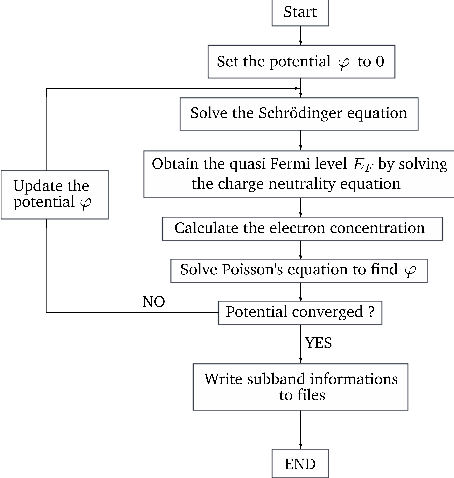
For a given Ns , the quasi Fermi level EF is obtained iteratively by solving equation (3.16). Both, the Schrödinger and the Poisson equations are discretized using the finite difference method. The procedures for the selfconsistent calculations are illustrated in Figure 3.1.