3.4.3 Semi-Empirical Method

Another method used to investigate the void evolution phenomenon caused by electromigration in interconnects is derived from a semi-empirical approach. Semi-empirical models for void evolution offer analytical expressions of measurable quantities (electrical resistance, time-to-failure,etc.) derived partially from theoretical aspects and partially obtained from experimental observations or by fitting to experimental results. The main difference from the void surface evolution models described previously is that semi-empirical methods involve approximations and assumptions in the physical theory, behind the model itself, in order to simplify the numerical calculation or to yield a result in accordance with experimental observations.

In this section, a semi-empirical analytical model describing the time required to grow a void in a passivated metal line, based on the void size dependence of the incoming flux of vacancies due to electromigration, is presented. The development of the model is mainly based on experimental studies presented in the work of Frank et. al [60].

In Section 3.2, the general expression of the vacancy flux responsible for electromigration failure in a metal line was obtained from equation (3.24). It has been shown that the electromigration force is the most dominant driving force in the vacancy flux responsible for the electromigration void evolution failure [118]. Therefore, in this context the other flux terms in equation (3.24), representing the components of the back-flux [16], can be neglected. The vacancy flux driven by electromigration can be written as

\[\begin{equation} \vec J_\text{v} = \cfrac{D_\text{v}C_\text{v}|Z^*|e\rho_\text{e}\vec j}{k_\text{b}T}, \end{equation}\] (3.90)

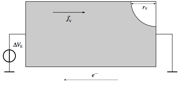
where ρ_e is the electrical resistivity of the metal. The vacancy flux induces the void nucleation in the section of the interconnect, where the highest vacancy flux divergence is expected. The flow of electric current transports the vacancies towards this region, where they are captured at the void surface. They may diffuse along the void surface, causing the void to grow. The void volume V_v change in time, due to the captured vacancies at the void surface, is given by

\[\begin{equation} \cfrac{\partial V_\text{v}}{\partial t} = f\Omega_\text{a} A_\text{i} ||{\vec{J_\text{v}||}} = f\Omega_\text{a} A_\text{i}\cfrac{D_\text{v}C_\text{v}|Z^*|e\rho_\text{e}||{\vec{j}}||}{k_\text{b}T}, \end{equation}\] (3.91)

where A_i is the cross sectional area of a given interconnect. Considering the case of an initial spherical void spanning the line ((3.11)), it is possible to approximate its evolution and local geometric features; a quarter-spherical void grows as

\[\begin{equation} \cfrac{\partial V_\text{v}}{\partial t} = \pi r_\text{v}^2 \cfrac{\partial r_\text{v}}{\partial t}, \end{equation}\] (3.92)

where r_v is the radius of the void.

Figure 3.11: Schematic cross section view of a conducting metal line with an initial small void of radius r_v.

Using equations (3.91) and (3.92), the void radius change in time is expressed as

\[\begin{equation} \cfrac{\partial r_\text{v}}{\partial t} = f\Omega_\text{a} A_\text{i}\cfrac{e|Z^*|D_\text{v}C_\text{v}\rho_\text{e}||{\vec{j}}||}{\pi r_\text{v}^2 k_\text{b}T}. \end{equation}\] (3.93)

The flux of vacancies captured by the void surface strongly depends on the void size, additionally influencing the changes in current density and vacancy concentration distributions around the void itself [45]. Assuming a variable vacancy flux and integrating equation (3.93), the analytical model describing the time t necessary to grow a void with a given radius becomes

\[\begin{equation} t = t_\text{0} + \cfrac{\pi}{ \alpha}\int_{r_\text{0}}^{r} \cfrac{r_\text{v}^2}{A_\text{i}(r_\text{v})C_\text{v}(r_\text{v})||{\vec{j}(r_\text{v})}||}\, \text{d}{r_\text{v}}, \end{equation}\] (3.94)

where

\[\begin{equation} \alpha = f\Omega_\text{a} \cfrac{e|Z^*|D_\text{v}\rho_\text{e}}{k_\text{b}T} , \end{equation}\] (3.95)

and r₀ is the initial void radius corresponding to time t₀.

By following the described modeling approach, an initial spherical void is placed at the location of void nucleation and its radius is increased. The time necessary to grow a void of a given volume can be obtained by performing numerical simulations of the vacancy flux around the void for different void sizes and applying equation (3.94).