4.2.3 Derivation of Equations over an Element

The derivation of algebraic equations in a finite element approach associated with the model DE, defined by equations (4.1) and (4.2), over a mesh element involves a three-step approach [125]:

1. Construction of the weak formulation of the DE;
2. Choice of the form of the approximate solution over the finite element;
3. Derivation of the finite element equations in matrix form by substituting the approximate solution into the weak formulation.

In the following, the construction of the algebraic equations over the isolated element Ω₁ with two nodes 1 and 2, whose endpoints have coordinates x=x₁ and x=x₁, is presented.

Step 1 - Weak Formulation

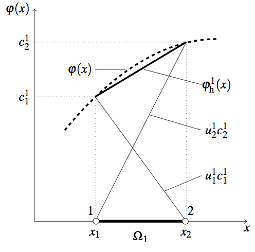
Different variational methods, such as the Ritz-Galerkin and weighted-residual, provide a background for the development of the algebraic equations over the element [116]. In all these methods, the basic idea is to seek a polynomial approximation φ_h¹ of the solution to equation (4.1) within the finite element Ω₁ in the form

\[\begin{equation} \varphi^{1}_\text{h}= \sum_{k=1}^{2} c^{1}_\text{k}u^{1}_\text{k}(x), \end{equation}\] (4.3)

where c_k¹ are the unknown nodal values of the solution φ(x)) at the nodes of the element Ω₁ and u_k¹ are the basis functions over the element. The scope of any variational method is to determine the nodal values c_k¹ in order to find an approximate solution φ_h¹ that best satisfies the DE at every point of the element Ω₁ of interest. The strong solution to equation (4.1) must be as smooth as required by the DE. In the present case, the solution should be continuously differentiable until at least the second derivative. To avoid such a requirement, the weak formulation of the problem is introduced. The main advantage compared to the strong form is that the weak form lowers the demand on continuity of the solution to only the first derivative.

The construction of the weak formulation of the problem requires one to recast the DE in a weighted-integral form [125]. The weighted-integral statement of the DE is constructed as follows

\[\begin{equation} \int_{x_\text{1}}^{x_\text{2}} w_\text{j}(x)R(x,c^{1}_\text{k}) \text{d} x=0,\quad \text{for} \quad j=1,2,...,n, \end{equation}\] (4.4)

where

\[\begin{equation} R(x,c^{1}_\text{k})=-\frac{d}{dx}\left(a\frac{d{\varphi^{1}_\text{h}}}{dx}\right) +b\varphi^{1}_\text{h}-f. \end{equation}\] (4.5)

R(x,c_k¹) is called residual of approximation of the DE within the element Ω₁ and w_j(x) is the weight function. The integral statement of equation (4.4) allows one to choose n linearly independent functions w_j(x) and obtain a set of n equations for c_k¹ by making R(x,c_k¹) equal to zero at the selected points of the element. It therefore requires that the basis function u_k¹ be such that the approximate solution φ_h¹ is twice differentiable. Note that the weighted-integral statement of (4.4) is equivalent to the DE and does not include any boundary conditions. The boundary conditions will come into play subsequently.

Due to the different choices of the weight function w_j(x) and/or the basis function u_k¹, the system of algebraic equations within the element will have different characteristics when different variational methods are used [125]. A general weighted-residual method is a variational method which requires only the weighted-integral statement of the DE to determine the nodal values c_k¹ of the approximation. The weight functions w_j(x) can be chosen from an independent set of functions, but are required to be linearly independent, otherwise the set of n equations for c_k¹ will not be solvable due to the underdetermination of the system of equations [88]. The Ritz-Galerkin method is a weighted-residual method which uses a set of weight functions w_j(x) equal to the set of basis functions u_k¹ such that the weighted-integral statement (4.4) reduces to

\[ \begin{equation} \int_{x_\text{1}}^{x_\text{2}} u_\text{j}(x)\left[-\frac{d}{dx}\left(a\frac{d{\varphi^{1}_\text{h}}}{dx}\right) +b\varphi^{1}_\text{h}-f\right] \text{d} x=0,\quad\text{for}\quad j=1,2,...,n. \end{equation}\] (4.6)

The weighted-residual approach provides residual minimization by integrating over the element. Using the integration by parts [148], the order of differentiation in φ_h¹ is reduced as follows

\[\begin{equation} \int_{x_\text{1}}^{x_\text{2}}\left(a\frac{d{u_\text{j}(x)}}{dx}\frac{d{\varphi^{1}_\text{h}}}{dx}+bu_\text{j}(x)\varphi^{1}_\text{h}\right) \text{d} x=\int_{x_\text{1}}^{x_\text{2}}u_\text{j}(x)f \text{d} x+\left[au_\text{j}(x)\frac{d{\varphi^{1}_\text{h}}}{dx}\right]_{x_\text{1}}^{x_\text{2}}. \end{equation}\] (4.7)

In this way, it is necessary that the basis functions u_k¹ be such that the approximate solution φ_h¹ is only once-differentiable, and not twice differentiable as in equation (4.6). Equation (4.7) represents the weak formulation of the problem. The term "weak" refers to the reduced or weakened continuity of u_k¹ such that φ_h¹ is differentiable as many times as called for the original DE in the weighted-integral statement [125].

Step 2 - Approximate Solution

The approximate solution φ_h¹ within the finite element Ω₁ must be found in a way that the approximate solution of the problem φ_h is convergent to the actual solution φ as the number of elements increase. For this purpose it is required to satisfy the following conditions [125]:

• Continuous over the element and differentiable, in order to ensure a regular coefficient matrix;
• Complete polynomial which includes all lower-order terms;
• Equal at both sides of each element node, so that the continuity of the solution is enforced when approximate solutions from each element are connected;
• Satisfy all the boundary conditions of the problem.

Consider the element Ω₁ composed of two nodes at x₁ and x₂, as depicted in (4.3).

Figure 4.3: Schematic view of the linear finite element approximation. The true solution φ(x) (dotted line) and the construction of the approximate solution φ_h¹ (solid line), within the element Ω₁, are presented.

Since only the first derivatives of φ_h¹ are involved in equation (4.7), the solution φ_h¹ within the element Ω₁ is approximated using a linear polynomial as follows

\[\begin{equation} \varphi^{1}_\text{h}(x)=g^{1}_\text{1}+g^{1}_\text{2}x\quad\quad x_\text{1}\leq x\leq x_\text{2}, \end{equation}\] (4.8)

where g₁¹ and g₂¹ are unknown coefficients. The expression (4.8) fulfills the first two conditions of an approximation described above. The third condition is satisfied if the unknown coefficients g₁¹ and g₂¹ are expressed in terms of nodal values of the solution φ₁¹(x₁) and φ₂¹(x₂). The nodal values are given by

\[\begin{align} \varphi^{1}_\text{1}(x_\text{1})=c^{1}_\text{1}=g^{1}_\text{1}+g^{1}_\text{2}(x_\text{1}),\\ \varphi^{1}_\text{2}(x_\text{2})=c^{1}_\text{2}=g^{1}_\text{1}+g^{1}_\text{2}(x_\text{2}). \end{align}\] (4.9)

By solving the system of equations (4.9) and using h₁=x₂-x₁, the unknown coefficients can be obtained as follows

\[\begin{align} g^{1}_\text{1}=\cfrac{c^{1}_\text{1}x_\text{2}-c^{1}_\text{2}x_\text{1}}{h_\text{1}},\\ g^{1}_\text{2}=\cfrac{c^{1}_\text{2}-c^{1}_\text{1}}{h_\text{1}}. \end{align}\] (4.10)

The substitution of equations (4.10) into equation (4.8) permits one to approximate the solution within the element as follows

\[\begin{align} \varphi^{1}_\text{h}(x)=\cfrac{c^{1}_\text{1}x_\text{2}-c^{1}_\text{2}x_\text{1}}{h_\text{1}}+\cfrac{c^{1}_\text{2}-c^{1}_\text{1}}{h_\text{1}}=\cfrac{x_\text{2}-x_\text{1}}{h_\text{1}}c^{1}_\text{1}+\cfrac{x-x_\text{1}}{h_\text{1}}c^{1}_\text{2}=u^{1}_\text{1}(x)c^{1}_\text{1}+u^{1}_\text{2}(x)c^{1}_\text{2}=\sum_{k=1}^{2}u^{1}_\text{k}(x)c^{1}_\text{k}, \end{align}\] (4.11)

where u₁¹(x) and u₂¹(x) are the basis functions or interpolation functions [116].

The interpolation property of these functions requires that u_k¹(x) is unity at the k^th node and zero at the other node of the given element. Another property of the interpolation functions is that their sum is unity. In this way, the solution φ_h¹(x) is interpolated using its nodal values c₁¹ and c₂¹, is approximated by a piecewise linear polynomial, and its gradient is constant within the element. The geometric representation of the approximate solution inside the element Ω₁ is shown in (4.3).

Step 3 - Ritz-Galerkin Method

Once the form of the approximate solution φ_h¹ within the element Ω₁ is known, the application of the Ritz-Galerkin method allows one to derive the set of algebraic equations over the finite element. The substitution of equation (4.11) into equation (4.7) will give the set of equations among the nodal values of the element as follows

\[\begin{equation} \sum_{k=1}^{2}\left[\int_{x_\text{1}}^{x_\text{2}}\left(a\frac{d{u_\text{j}(x)}}{dx}\frac{d{u^{1}_\text{k}}}{dx}+bu_\text{j}(x)u^{1}_\text{k}\right) \text{d}x\right] c^{1}_\text{k}=\int_{x_\text{1}}^{x_\text{2}}u_\text{j}(x)f \text{d}x+\sum_{k=1}^{2}u_\text{j}(x_\text{k})\beta^{1}_\text{k}, \end{equation}\] (4.12)

where

\[\begin{equation} \beta^{1}_\text{k}=\left(a\frac{du^{1}_\text{k}}{dx}\right)\Bigg|_{x=x_\text{k}} \end{equation}\] (4.13)

are the unknown source terms. Usually, such a relation for the finite element Ω₁ is presented as a matrix equation [161] of the form

\[\begin{equation} [K^{1}]\{c^{1}\}=\{f^{1}\}+\{\beta^{1}\}, \end{equation}\] (4.14)

where

\[\begin{equation} [K^{1}]=\int_{x_\text{1}}^{x_\text{2}}\left(a\frac{du_\text{j}(x)}{dx}\frac{du^{1}_\text{k}}{dx}+bu_\text{j}(x)u^{1}_\text{k}\right)\text{d}x, \end{equation}\] (4.15)

\[\begin{equation} \{f^{1}\}=\int_{x_\text{1}}^{x_\text{2}}u_\text{j}(x)f dx, \end{equation}\] (4.16)

and

\[\begin{equation} \{\beta^{1}\}=\sum_{k=1}^{2}u_\text{j}(x_\text{k})\beta^{1}_\text{k}. \end{equation}\] (4.17)

The matrix [K¹], which is called coefficient matrix, and the vector {f¹}, which is the source vector, can be determined for the given element and known functions a, b, and f. The relation (4.14) provides two equations for the finite element used to determine four unknowns: c₁¹, c₂¹, β₁¹, and β₂¹. For a linear element, the matrix form is written as follows

\[\begin{equation} \begin{bmatrix} K^{1}_\text{11} & K^{1}_\text{12} \\[2pt] K^{1}_\text{21} & K^{1}_\text{22} \\ \end{bmatrix} \begin{Bmatrix} c^{1}_\text{1} \\[2pt] c^{1}_\text{2} \\ \end{Bmatrix} = \begin{Bmatrix} f^{1}_\text{1} \\[2pt] f^{1}_\text{2} \\ \end{Bmatrix} +\begin{Bmatrix} \beta^{1}_\text{1} \\[2pt] \beta^{1}_\text{2} \\ \end{Bmatrix}, \end{equation}\] (4.18)

where the coefficients of the matrix (K_jk¹) and the source vector (f_j¹) can be easily evaluated for the given element from equations (4.15) and (4.16), respectively, by using the values of the constants a, b, and f.