4.2.4 Assembly of Elements

Equation (4.14) can not be solved without using the equations from other finite elements [125]. The assembling of elements is a method to obtain the equations for the complete set of elements of the total problem [161]. The connectivity of elements provides the finite element equations of the total problem by putting the elements back into their original position in order to get rid of the extra unknowns [125]. For this purpose, the procedure requires that the solution is continuous and the unknown source terms β_kⁱ are balanced at nodes common to several elements where they are connected to each other.

Consider the simple case of two linear elements Ω₁ and Ω₂ connected at the node 2, as shown in (4.4).

Figure 4.4: Schematic view of the assembly of two linear elements Ω₁ and Ω₂. The definition of the boundary conditions at the endpoints, the balance of the unknown source terms, and the continuity of the solution at node 2 are presented.

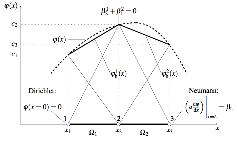For a mesh of linear finite elements, the continuity of the solution requires that node 2 of the element Ω₁ is connected to node 2 of the element Ω₂ such that c₂¹=c₁²=c₂, where c₂ is the unknown nodal value at the common nodal point. For the same mesh of elements, the balance of the unknown source terms β_kⁱ at connecting nodes requires that

\[\begin{align} \beta^{1}_\text{2}+\beta^{2}_\text{1} = \begin{cases}0 & \mbox{} \text{if no external source is applied}\mbox{}, \\ \beta_\text{f} & \mbox{} \text{if an external source is applied}\mbox{}, \end{cases} \end{align}\] (4.19)

where β_f is the magnitude of the external applied source.

Considering the case of two linear elements and adopting relation (4.14), the matrix form for the algebraic equations of the elements Ω₁ and Ω₂ are

\[\begin{equation} \begin{bmatrix} K^{1}_\text{11} & K^{1}_\text{12} \\[2pt] K^{1}_\text{21} & K^{1}_\text{22} \\ \end{bmatrix} \begin{Bmatrix} c^{1}_\text{1} \\[2pt] c^{1}_\text{2} \\ \end{Bmatrix} = \begin{Bmatrix} f^{1}_\text{1} \\[2pt] f^{1}_\text{2} \\ \end{Bmatrix} +\begin{Bmatrix} \beta^{1}_\text{1} \\[2pt] \beta^{1}_\text{2} \\ \end{Bmatrix}, \end{equation}\] (4.20)

and

\[\begin{equation} \begin{bmatrix} K^{2}_\text{11} & K^{2}_\text{12} \\[2pt] K^{2}_\text{21} & K^{2}_\text{22} \\ \end{bmatrix} \begin{Bmatrix} c^{2}_\text{1} \\[2pt] c^{2}_\text{2} \\ \end{Bmatrix} = \begin{Bmatrix} f^{2}_\text{1} \\[2pt] f^{2}_\text{2} \\ \end{Bmatrix} +\begin{Bmatrix} \beta^{2}_\text{1} \\[2pt] \beta^{2}_\text{2} \\ \end{Bmatrix}, \end{equation}\] (4.21)

respectively. For a mesh of two linear finite elements connected in series, the interelement continuity of the solution requires that

\[\begin{equation} c^{1}_\text{1}=c_\text{1},\, c^{1}_\text{2}=c^{2}_\text{1}=c_\text{2},\, c^{2}_\text{2}=c_\text{3}, \end{equation}\] (4.22)

and the balance of the unknown source terms at the global points, in this case only node 2, is interpreted as follows

\[\begin{equation} \beta^{1}_\text{2}+\beta^{2}_\text{1}=0. \end{equation}\] (4.23)

The second equation of the matrix (4.20) for the element Ω₁ must be added to the first equation of the matrix (4.21) for the element Ω₂, in order to reduce the number of equations from 2N to N+1 in a mesh of N linear elements. In terms of the global nodal values, the sum of equation (4.20) and equation (4.21) results in the assembled global equation system for the domain with two elements and three nodes as follows

\[\begin{equation} \begin{bmatrix} K^{1}_\text{11} & K^{1}_\text{12} & 0 \\[2pt] K^{1}_\text{21} & K^{1}_\text{22}+K^{2}_\text{11} & K^{2}_\text{12} \\[2pt] 0 & K^{2}_\text{21} & K^{2}_\text{22} \\ \end{bmatrix} \begin{Bmatrix} c_\text{1} \\[2pt] c_\text{2} \\[2pt] c_\text{3} \\ \end{Bmatrix} = \begin{Bmatrix} f^{1}_\text{1} \\[2pt] f^{1}_\text{2}+f^{2}_\text{1} \\[2pt] f^{2}_\text{2} \\ \end{Bmatrix} +\begin{Bmatrix} \beta^{1}_\text{1} \\[2pt] 0 \\[2pt] \beta^{2}_\text{2} \\ \end{Bmatrix}. \end{equation}\] (4.24)

These are called assembled equations, which contain the sum of coefficients and source terms at the global point to two elements. The assembly matrix contains three equations in five unknowns: c₁, c₂, c₃, β₁¹, and β₂².