Basis Functions and Domain Partitioning

3.1.4 Basis Functions and Domain Partitioning

In principle, there are no restrictions to choose the basis functions of the space $V h$ . Nevertheless, the complexity of the linear system (3.14) is defined by them. The quality of the approximated solution $uh$ is expected to increase with the increased dimension of $Vh$ [59]. Thus, good approximations lead to big matrices (A) and consequently to the increase in the computational costs of solving (3.14). From a pragmatic point of view, a sparse matrix A would diminish the computational burden of a high-dimensional $Vh$ space. An ingenious choice of basis function should create sparse matrices while keeping the requirements for a good approximation.

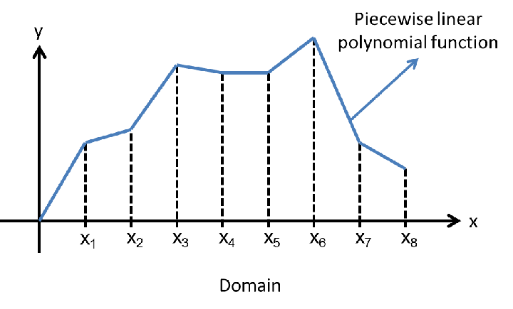
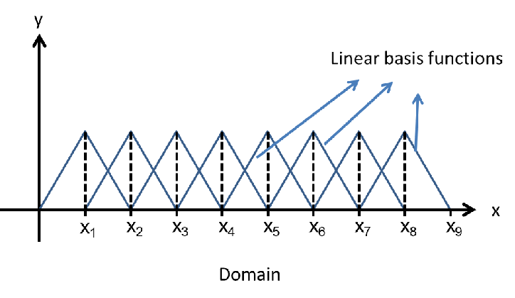
Polynomial piecewise functions are the most traditional choice for basis functions in FEM [56][57]. They are defined in a particular way such that the domain needs to be partitioned as in Fig. 3.3. Each partition is known as a finite element (the origin of the method name). In each element, a set of basis function is defined according to the following criteria [57]:

It assumes a non-zero value at a node i. In all other nodes the function is zero. Therefore, one function per node.
It vanishes over all the elements which contain the node i, following the established polynomial rule.
It must be an element of $Vh$ , therefore it must be continuous and must have the first derivative be piecewise continuous.

pict

Figure 3.1.:

A set of linear basis functions of $Vh$ . As the number of partitions increases, the amount of functions which are possible to represent the solution ( $Vh$ dimension) also increases. As consequence, the quality of the approximation is enhanced.

This guidance enables the creation of sparse matrices and simplifies the post-processing of the solution. In Fig. 3.2 a linear piecewise basis function is depicted, which was constructed following the aforementioned criteria.

pict

Figure 3.2.:

Linear basis function constructed according to the presented criteria.

The construction of basis functions has been a process developed and refined along the years to minimize the computational costs of FEM [57]. It is clear from the criteria that the pattern of the basis function will repeat along the elements. The polynomial in Fig. 3.3 can be generated by linear basis functions as in Fig. 3.2.

pict

Figure 3.3.:

An example of a piecewise linear polynomial function. For each partition a linear function is defined.

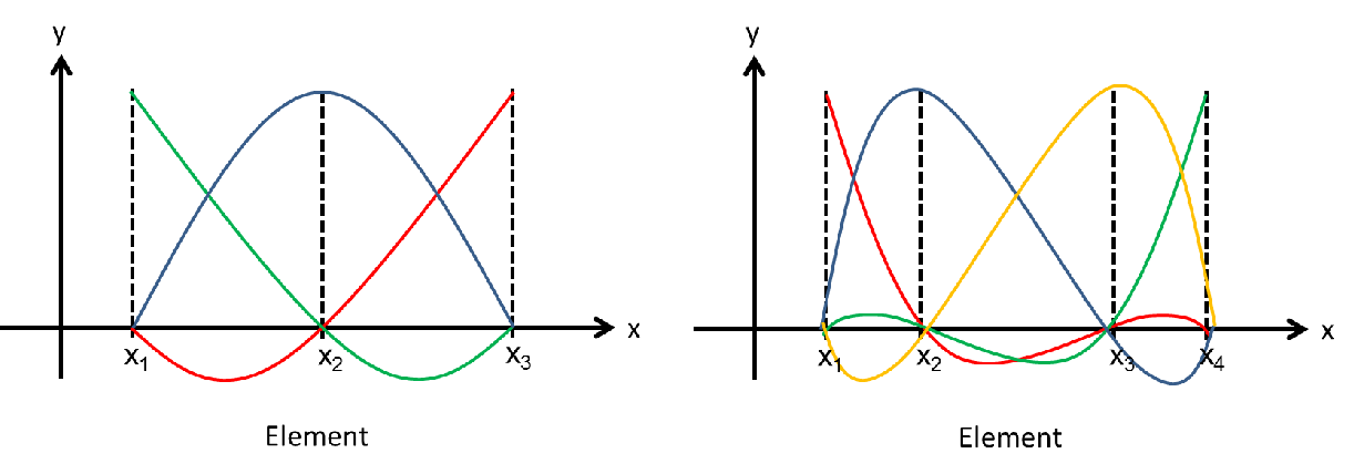
Usually, nodes are defined by the boundaries of the element, but some basis functions may require additional nodes. Those points do not define the boundaries, instead they are used as control points. Higher degree polynomials basis functions are created in this fashion, while they also must follow the criteria. In Fig. 3.4, basis functions with quadratic and cubic polynomials are exemplified.

pict

Figure 3.4.:

Quadratic (left) and cubic (right) basis function.

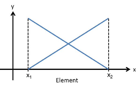
As sample application, consider the partition of the BVP problem (3.1) discussed so far. Let linear piecewise polynomials be the basis functions as in Fig. 3.1. Analytically, the linear piecewise basis function can be defined by

( { 1∕hj [xj− 1,xj] ϕj = (− 1∕hj+1 [xj,xj+1 ] , 0 (x < xj−1)∪ (x > xj+1)

(3.15)

where $hj$ is the size of the element as described in Fig. 3.2. As seen before, the discrete variational formulation of the BVP problem leads to the linear system (3.14). In order to solve the system, a computation of $∫ ϕ′iϕ′jdx$ is required. For the basis functions employed here this task is straightforward. If $|i − j| > 1$ then $∫ ϕ′iϕ′jdx = 0$ , since whenever $|i− j| > 1$ or $ϕx(x)$ or $ϕj(x)$ the solution is zero. In the cases of $|i− j| < 1$ the integration result for $i = j$ is given by

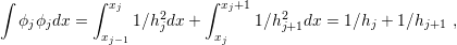∫ ∫ ∫ xj 2 xj+1 2 ϕj ϕjdx = xj−1 1∕hjdx + xj 1∕hj+1dx = 1∕hj + 1∕hj+1 ,

(3.16)

while the result for $i = j − 1$ and $i = j + 1$ is given by

∫ ∫ ∫ xj ϕjϕj + 1dx = ϕj ϕj − 1dx = − 1∕h2jdx = − 1∕hj . xj−1

(3.17)

Assuming a homogeneous partition of the domain ( $1∕hj = 1∕hj−1$ ) (3.14) can be rewritten as

⌊ ⌋⌊ C ⌋ ⌊ ∫ f ϕ dx⌋ | 2 − 1 0 ⋅⋅⋅ ⋅⋅⋅ 0 || .1| | .1 | |− 1 2 − 1 0 ⋅⋅⋅ 0 ||| .. || || .. || || 0 ... ... ... ... ... |||| .. || || .. || || . . . . . . |||| . || = || . || . || .. .. .. .. .. .. ||| ... | | ... | |⌈ .. ... ... ... ... |⌉|| .. || || .. || . − 1 ⌈ . ⌉ ⌈∫ . ⌉ 0 ⋅⋅⋅ ⋅⋅⋅ 0 − 1 2 CN fϕN dx

(3.18)

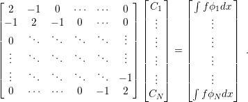
The linear system (3.18) is the final discretized form of the original BVP problem (3.1). The matrix is sparse due to the choice of the basis functions, and it is also symmetric, which is a great advantage for computing the solution of the system. Symmetry is a desirable property which is very dependent on the problem, but the right choice of the basis functions can ensure it for the linear system.

The development made so far is only suitable for differential equations in the same form as described in (3.1), including the boundary conditions. The problem (3.1) is rather common in nature. Heat transfer, elasticity, and electrostatics are examples of phenomena described by it. The choice here was motivated by the use of (3.1) for different fields and the importance to the models used in this work. Naturally, another differential equation will lead to another variational form. However, the idea remains the same: to multiply it by a function of the space $V$ , to integrate it over the domain, to discretize it by $Vh$ , to partition the domain, to choose the basis functions, and finally to solve the system, summarizing the steps for finding a solution using the Finite Element Method.

Considerations for 2D and 3D Cases

For 2D and 3D problems the procedure is the same, while the mathematical semantics and operations (derivatives and integrations) must be adapted for the proper dimension. The main difference lies in the partitioning of the domain, which can be split in different ways. The creation procedure of a partition is called meshing and the resultant domain division is a mesh. There are several algorithms available for meshing, however, the vast majority of them creates triangular or quadrilateral meshes for 2D domains and tetrahedral and quadrilaterally-faced hexahedral meshes for 3D domains [60].

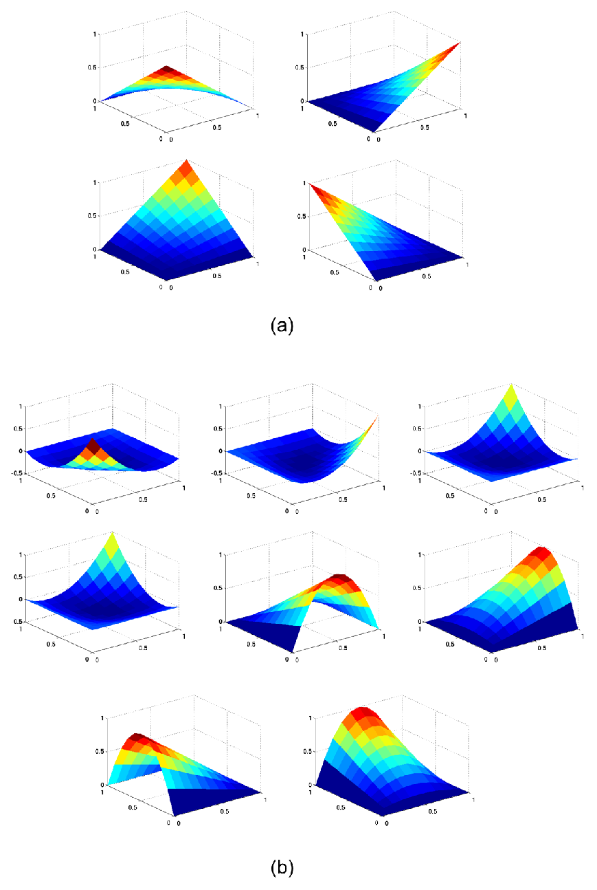
Regarding the basis functions, the concept for creation persists. The criteria for construction should still be satisfied and they should be polynomials, but for this case in 2D and 3D dimensions. The basis functions construction for 2D and 3D domains is rather lengthy and cumbersome, however, well treated in a variety of textbooks [56][57]. Examples of basis functions for 2D domains with quadratic meshes are detailed in Fig. 3.5.

pict

Figure 3.5.:

Basis functions defined in 2D domains. Linear (a) and quadratic (b) functions in quadrilateral domains.

[next] [prev] [prev-tail] [front] [up]