The storage of data related to geometric objects like points or
facets is part of the following considerations. Due to different appearances
of the overall terminus ``data'' a specification is given towards the
class of ![]() -dimensional tensors in general with emphasis on three-dimensional
tensors up to a rank of two. The data - geometric object relation is
explained by means of all faces of a
-dimensional tensors in general with emphasis on three-dimensional
tensors up to a rank of two. The data - geometric object relation is
explained by means of all faces of a ![]() -simplex.
-simplex.
An
![]() rank tensor in
rank tensor in ![]() -dimensional space is a mathematical
object that has
-dimensional space is a mathematical
object that has ![]() indices and
indices and ![]() components. Each index
of a tensor ranges over the number of dimensions of space. Tensors are
generalizations of scalars (that have no indices), vectors (that have exactly
one index), and matrices (that have exactly two indices) to an arbitrary number
of indices [54].
components. Each index
of a tensor ranges over the number of dimensions of space. Tensors are
generalizations of scalars (that have no indices), vectors (that have exactly
one index), and matrices (that have exactly two indices) to an arbitrary number
of indices [54].
Depending on the rank of the tensor different numbers of components can be
counted for one data value in three-dimensional space. It is known that
a scalar has only a magnitude and no directional part, so there is only one
component for a scalar data value. A tensor of rank one, which is also known as
vector, consists of one direction and a magnitude, which gives three
components for one vector data value. For a dyad which is a tensor of rank
two, two directions and one magnitude is counted which gives nine components for
a dyad data value [55]. This list of course can be extended ad
infinitum, but for this work it is sufficient to stop at tensors of rank two.
Section A.3 shows how tensors of rank two can be visualized by a so called glyph representation. Figure 3.1(a) and Figure 3.1(b) show also glyph visualization for tensors of rank zero and one, respectively.
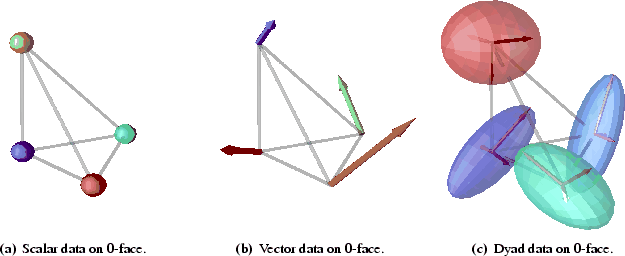 |
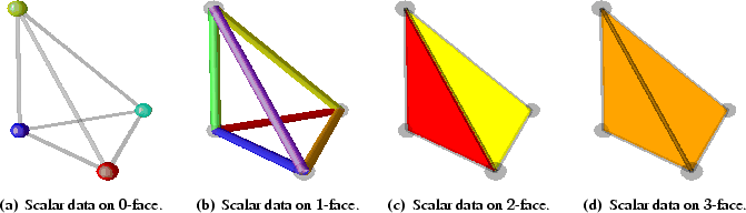
Figure 3.2 shows four different data ![]() -face relations of a
-face relations of a
![]() -simplex. Data values can be stored related to the 0
-face (vertices),
-simplex. Data values can be stored related to the 0
-face (vertices),
![]() -face (edges),
-face (edges), ![]() -face (facets), and
-face (facets), and ![]() -face (
-face (![]() -simplex or
tetrahedron), cf. Figure 3.2(a) - 3.2(d),
respectively. Depending on the
-simplex or
tetrahedron), cf. Figure 3.2(a) - 3.2(d),
respectively. Depending on the ![]() -face data relation different number of
values can be associated, e.g. for a 0
-face data relation, four data values
are needed (one for each vertex) and for a
-face data relation different number of
values can be associated, e.g. for a 0
-face data relation, four data values
are needed (one for each vertex) and for a ![]() -face relation only one data
value is needed which is constant over the whole volumetric simplex.
-face relation only one data
value is needed which is constant over the whole volumetric simplex.
As seen in Section 3.1.2 different data ![]() -face relations are possible
on tetrahedral meshes. One has to say that for further investigations two
relations are important, namely the data 0
-face (cf. Figure 3.2(a)),
and the data
-face relations are possible
on tetrahedral meshes. One has to say that for further investigations two
relations are important, namely the data 0
-face (cf. Figure 3.2(a)),
and the data ![]() -face relation (cf. Figure 3.2(d)). Since the data
values are constant over the whole mesh element (
-face relation (cf. Figure 3.2(d)). Since the data
values are constant over the whole mesh element (![]() -simplex) for a
-simplex) for a ![]() -face
relation, no data interpolation over the element is necessary.
-face
relation, no data interpolation over the element is necessary.
For tetrahedral meshes with data values stored in 0
-face relation, the
situation is slightly different and one has to think about interpolation of those
scattered data, to obtain a more or less continuous data field which is
essential for further numerical calculations or at least for
visualization. The choice of the interpolation method depends on
the underlying numerical discretization scheme and should be carried out with
care.
Based on some ideas of finite element calculations an interpolation scheme is
presented in the following, which allows linear interpolation over the
![]() -simplex that is value conformal at the vertices.
-simplex that is value conformal at the vertices.
A canonical map from the standard ![]() -simplex to an arbitrary
-simplex to an arbitrary
![]() -simplex with vertices
-simplex with vertices
![]() is given by
is given by
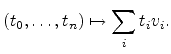 |
(3.1) |
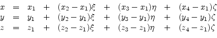
The following coordinate transformation
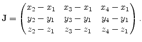
In matrix notation Equation (3.2) can be written as
| (3.3) |
 |
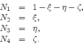
The idea behind this interpolation scheme is to construct a continuous data
distribution from 0
-face data values with the help of so-called weighting
functions. The definition of this functions is given for the standard
![]() -simplex with the coordinates
-simplex with the coordinates
![]() and can be easily mapped
onto every arbritrary
and can be easily mapped
onto every arbritrary ![]() -simplex as depicted above (see Figure 3.3).
-simplex as depicted above (see Figure 3.3).
The linear weighting functions for a standard ![]() -simplex read:
-simplex read:
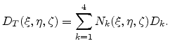
If the 0
-faces
![]() of a
of a ![]() -simplex
-simplex ![]() hold the data
values
hold the data
values
![]() , the continuous data distribution over
the
, the continuous data distribution over
the ![]() -simplex
-simplex ![]() mapped on the standard simplex can be written as:
mapped on the standard simplex can be written as:
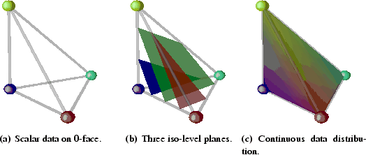
Figure 3.4 gives an impression on how this interpolation scheme acts
on arbitrary scalar data values. The iso-level planes shown in
Figure 3.4(b) are without any coverture and their transition from one
![]() -simplex to a possible neighboring
-simplex to a possible neighboring ![]() -simplex is in general not
differentiable, but always value conformal which is characteristic for
piecewise linear interpolation.
-simplex is in general not
differentiable, but always value conformal which is characteristic for
piecewise linear interpolation.
For higher order basis functions, the vertex points of the
standard ![]() -simplex plus additional sampling points have to be taken into
account. In [32] an overview of different basis functions, up to a
degree of two and for different mesh elements regarding the two- and
three-dimensional case are shown.
-simplex plus additional sampling points have to be taken into
account. In [32] an overview of different basis functions, up to a
degree of two and for different mesh elements regarding the two- and
three-dimensional case are shown.
![\includegraphics[width=0.75\textwidth]{pics/tet-map.eps}](img194.png)
![$\displaystyle \mathbf{J}= \begin{pmatrix}\frac{{\rule[0.0mm]{0mm}{\Myhi}\displa...
...m]{0mm}{\Myhi}\displaystyle\partial \zeta}} \rule[-3mm]{0mm}{7mm} \end{pmatrix}$](img200.png)