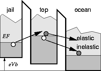
Figure 3: Co-tunneling via a virtual intermediate state.

An electron can not tunnel directly from jail to ocean. Also a
normal tunneling from jail to top is impossible
because of missing thermal energy. Nevertheless, an electron will escape
to ocean via an intermediate virtual state. One could also picture this
process in the following simplified way. An electron starting at jail
overcomes the energy difference to top for a very short time allowed by
Heisenberg's uncertainty principle. If a different electron from top tunnels
in the same very short time to ocean, then overall an electron escaped from
jail to ocean. This process is called the inelastic co-tunnel effect.
There is another usually negligible process, which is called elastic
co-tunneling, where the same electron that tunneled first from jail to
top, tunnels further to ocean. In this case the phase of the electron is
preserved, which makes elastic co-tunneling a coherent process.
Elastic co-tunneling strongly depends on the internal structure of the
island. Usually inelastic co-tunneling is dominant in comparison to
elastic co-tunneling except at very small bias voltages and temperatures
or very low energy state densities in the quantum dot
[16].
The rate of second order inelastic co-tunneling can be written as [2] [3]
![]()
where ![]() represents the tunneling amplitude through barrier i,
represents the tunneling amplitude through barrier i,
![]() is the change in energy of the system for a tunnel event
through barrier i, and
is the change in energy of the system for a tunnel event
through barrier i, and ![]() and
and ![]() are the initial and final energies
of the system. A description of rate formulas of higher order
co-tunneling and a good approximation for the rate formulas can be found in
L. Fonseca et al.
[11]. Fonseca et al. study the
electron trap and show that co-tunneling is a major source of errors at
temperatures with thermal energies considerably lower than the
characteristic Coulomb blockade energy. Since single-electron devices have
to be operated at temperatures low enough for a clearly pronounced
Coulomb blockade, co-tunneling is the dominating error source.
are the initial and final energies
of the system. A description of rate formulas of higher order
co-tunneling and a good approximation for the rate formulas can be found in
L. Fonseca et al.
[11]. Fonseca et al. study the
electron trap and show that co-tunneling is a major source of errors at
temperatures with thermal energies considerably lower than the
characteristic Coulomb blockade energy. Since single-electron devices have
to be operated at temperatures low enough for a clearly pronounced
Coulomb blockade, co-tunneling is the dominating error source.
The usual approach to overcome the rare tunnel event problem is to use a ME method instead of a MC method, as was done by Fonseca et al. [11]. The master equation is given by
where ![]() is the tunnel rate between states i and j, and
is the tunnel rate between states i and j, and
![]() is the occupation probability of state i.
Although the ME gives theoretically accurate results even for very rare
tunnel events, it has many other
impracticabilities that limit its accuracy and usability. The starting
point of the ME is the set of all relevant states a circuit will occupy
during operation.
There is no straightforward way to obtain this set. In order
to achieve the desired simulation goal one has to include many more states
than would be relevant, which results in extremely long simulation times and
sometimes bad numerical stability. On the other side a MC method allows
an easy trade-off between accuracy and simulation time. Thus one can achieve
quick approximate results of very large circuits, which would otherwise
not be feasible to compute. Hence our desire was to stick with the MC
method profiting from its advantages, but on the other side being able
to simulate co-tunneling better than with the brute force method where
so many tunnel events are simulated that enough rare events are among them.
Anyway the brute force method is often because of extremely long simulation
times not possible.
is the occupation probability of state i.
Although the ME gives theoretically accurate results even for very rare
tunnel events, it has many other
impracticabilities that limit its accuracy and usability. The starting
point of the ME is the set of all relevant states a circuit will occupy
during operation.
There is no straightforward way to obtain this set. In order
to achieve the desired simulation goal one has to include many more states
than would be relevant, which results in extremely long simulation times and
sometimes bad numerical stability. On the other side a MC method allows
an easy trade-off between accuracy and simulation time. Thus one can achieve
quick approximate results of very large circuits, which would otherwise
not be feasible to compute. Hence our desire was to stick with the MC
method profiting from its advantages, but on the other side being able
to simulate co-tunneling better than with the brute force method where
so many tunnel events are simulated that enough rare events are among them.
Anyway the brute force method is often because of extremely long simulation
times not possible.

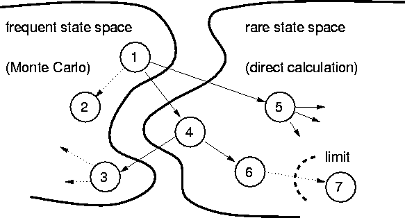
The MC part simulates only the frequent state space, which gives the
occupation probabilities of frequent states. The occupation probability
![]() is calculated as the
ratio of time
is calculated as the
ratio of time ![]() spent in
state i to the total simulation time
spent in
state i to the total simulation time
![]() .
.

The essential assumption is that the rare states cause only a small
perturbation to the frequent state probabilities.