Band structure

2.1 Band structure

In Equation (2.4) the kinetic energy operator and the periodic lattice potential have been replaced by the dispersion relations Eν(k) for ν bands. This enables us to treat an electron in a lattice as a free quasi-electron, where the first derivative of Eν(k) is related to the momentum p_ν and therefore the group velocity (cf. Equation (2.2)) and the second derivative of Eν(k) is related to the effective mass tensor m_ν^*

p_ν	= m₀vg = ∇kEν(k),	(2.5)
(m_ν^*)^-1	= .	(2.6)

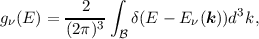In order to efficiently compute the electron and hole densities from Equation (2.16) the density of states (DOS) gν(E) is needed. The DOS can be calculated from the dispersion relation Eν(k) using [12]

∫ --2-- 3 gν(E) = (2π)3 δ(E - E ν(k))d k, B

(2.7)

where denotes the first Brillouin Zone (BZ) [16, 17, 14] (cf. Figure 2.1) in the band structure, shown for silicon in Figure 2.2, of the semiconductor. Most often in the analysis of semiconductors, the bands are separated in the middle of the band gap into conduction and valence bands for electrons and holes respectively. Thus also the DOS has to be separated into a DOS for electrons gnν(E) and holes gp ν(E). The so obtained DOS for silicon is shown in Figure 2.1.

Upon combining the definitions of the distribution function (Equation (2.16) and the DOS (Equation (2.7) one arrives at

∫ ∫ n = fνngnν(E )dE, p = fνpgpν(E)dE,

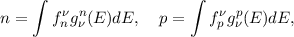(2.8)

to calculate the macroscopic electron n and hole p concentrations. As will become clearer later, n and p are moments of their respective BTE.

PICT

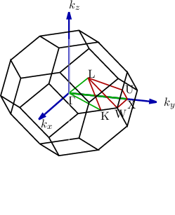
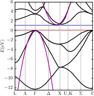
Figure 2.1:

Left: The first Brillouin zone (BZ) of silicon. The lines and points of symmetry are shown in red (on the edge of the BZ) and green (within the BZ). Right: The band structure of silicon from [18] calculated using a non-local pseudpotential method, which neglects spin-orbit interaction [19]. The conduction band edge is indicated by the blue line, whereas the red line indicates the valence band edge. The bandstructure as obtained by a parabolic approximation is also shown (purple).

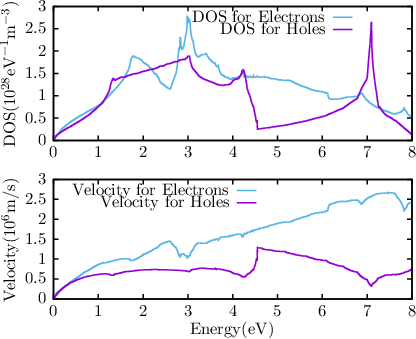
Figure 2.2:

The density of states (DOS) and group velocity for relaxed silicon used for the solution of the bipolar BTE.

Parabolic Band Approximation

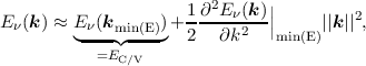
From Figure 2.1 one can easily deduce that, in the important case of silicon, there is no simple analytic expression for the bandstructure. This poses a fundamental problem for many approximations and solution techniques of the BTE, Monte Carlo methods being a notable exception. Thus analytic approximations for the bandstructure are sought. One of them is the parabolic band approximation. The main argument justifying this approximation is that for low and moderate fields the electrons still occupy states close to the band minimum. The parabolic band approximation is obtained by expanding the dispersion relation Eν(k) into a Taylor series. Upon evaluating the series for k at the lowest energy E one obtains

1 ∂2E ν(k )|| 2 E ν(k) ≈ Eν(kmin(E)) +2---∂k2---|min(E)||k||, ◟ =E◝◜ ◞ C∕V

(2.9)

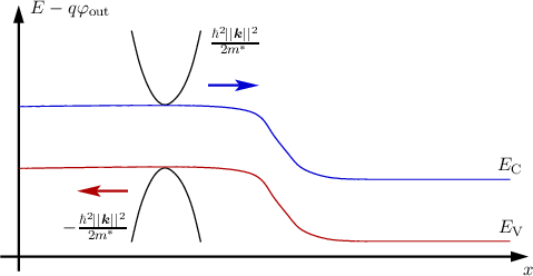
where the first term on the right hand side is a constant energy to account for the distance between the conduction band edge and the choice of the reference energy E_ref = 0 (cf. Figure 2.3).

Figure 2.3:

Sketch of the parabolic band approximation in a 1D device.

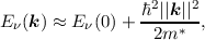
If the minimum energy is to be found at k = 0 then the above equation reduces to

2 2 E ν(k) ≈ E ν(0)+ ℏ-||k||-, 2m *

(2.10)

where the effective mass tensor (cf. Equation (2.6)) is assumed to be isotropic and scalar. However, in silicon this is not the case (cf. Figure 2.1) and the effective mass m^* is not isotropic as assumed in the equations above. For the conduction band in silicon, Equation (2.10) is often reduced to

2( 2 2 2 ) E(k) ≈ E + ℏ-- k-x + ky-+ kz- , C 2 my my mz

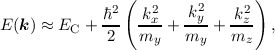(2.11)

where m_x, m_y and m_z are the components of the effective mass tensor m^* and we restricted ourselves to a single effective band. Sometimes the relation Equation (2.10) is favored over Equation (2.11), since a scalar k can be used instead of a vectorial k thereby simplifying the analysis. This can be achieved by the Herring-Vogt transform [20] without any further assumptions through a linear coordinate transform in k-space.

Kane’s Model

The parabolic band approximation is often used up to high energies at high fields were it obviously fails to predict the correct band structure (cf. Figure 2.1). In order to improve this the parabolic band approximation has been extended [21] to account for the non-parabolicity in the band structure by introducing the factor α for the first (conduction or valence) band as follows:

2 2 E(k)[1+ αE (k)] = ℏ-k-, 2m *

(2.12)

where α = 0.5 is a good choice for electrons in silicon.

[next] [prev] [prev-tail] [front] [up]