2.2 The Boltzmann Transport Equation
The Boltzmann Transport equation (BTE) has been originally developed by Ludwig Boltzmann to
statistically describe transport of atoms and molecules (particles) of an idealized diluted gas. The
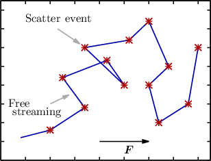
BTE describes the transport by two processes, namely free streaming and scattering. In order to use
the BTE to describe transport of an electron gas in a semiconductor, the BTE for diluted gases needs
to be modified. First the free streaming of the charge carriers in the lattice is described by the
equations of motion (Newton’s law)
 | (2.13) |
where the relation p = ℏk and the band structure is used. Second, to describe the collisions between
electrons in the electron gas, we will use quantum mechanical perturbation theory (Fermi’s Golden
Rule). It has to be noted that in the classical framework of the BTE, where Heisenbergs uncertainty
principle is being neglected, one could directly track position and momentum of each electron.
However, this tracking of each single particle in a classical approach is currently infeasible.
Instead we will modify the BTE as stated above, by rederiving the BTE using Equation (2.4).
Although the derivation of the BTE has been covered in many works before, its derivation will
nevertheless be repeated from [13, 12] for the sake of clarity. For this purpose we need to define a
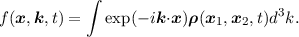
distribution function f(x,k,t) of the carriers in real- and reciprocal-space. The distribution function
f(x,k,t) is defined such that
 | (2.14) |
is the number of particles (electrons or holes) in the infinitesimal small volume d3xd3k in the
six-dimensional phase-space. The distribution function is a semi-classical concept, since it assumes
that both position and momentum of a particle can be measured to arbitrary accuracy at the same
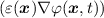
time. In order to introduce the semi-classical concept into the Hamiltonians of Equation (2.4), we
treat the electrons as classical particles governed by classical mechanics in the time intervals they
do not scatter with other particles. Thus the external force exerted on a single electron
is
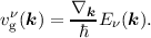
The group velocity vνg(k) can then be calculated [12] as
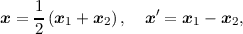
Starting from the definition of the density matrix
 | (2.15) |
we define the distribution function as the Fourier transformed density matrix
 | (2.16) |
This definition is compatible with the previous definition in Equation (2.14), since the
density matrix describes a statistical ensemble of quantum states in real space. In order to
transform the density matrix to the phase space, a Fourier transform needs to be carried out.
To asses the time evolution of the density matrix we utilize the Liouville-Von-Neumann
equation,
| (H(x1) - H(x2))ρ(x1,x2,t) = ∂tρ(x1,x2,t), | (2.17)
|
| ⇒ | iℏ∂tρ(x1,x2,t) + (Eν(-i∇x1) - Eν(-i∇x2) | (2.18)
|
| | - φout(x1,t) + φout(x2,t))ρ(x1,x2,t) = 0, | (2.19) |
where the simplified and approximated Hamilton-Operators from Equation (2.4) have been used.
Scattering will be neglected for the time being, since it will be treated as a perturbation later. After a
transformation of coordinates,
 | (2.20) |
the operators can be linearized by assuming that each electron is sharply distributed in k-space and
that the electrostatic potential changes over x are small compared to the changes of the electronic
wavefunction over x
| - φout(x1,t) + φout(x2,t) | ≈∇xφout((x2 + x1)∕2,t)⋅(x2 + x1) = 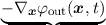 =F(x)∕q⋅x′ =F(x)∕q⋅x′ | (2.21)
|
| Eν(-i∇x1) - Eν(-i∇x2) | ⇒ iℏvν
g(-i∇x′)⋅∇x | (2.22) |
Inserting the above approximations into Equation (2.17) one obtains:
 | (2.23) |
Finally, a Fourier transformation of the equation above is carried out and one obtains after a few
algebraic rearrangements the well known homogeneous BTE for the νth band
 | (2.24) |
where  {fν(x,k,t)} is the free-streaming operator. In order to incorporate scattering processes
a semi-classical perturbation term
{fν(x,k,t)} is the free-streaming operator. In order to incorporate scattering processes
a semi-classical perturbation term  {fν(x,k,t)} on the right hand side of the BTE is
required
{fν(x,k,t)} on the right hand side of the BTE is
required
 | (2.25) |
{fν(x,k,t)} is obtained by perturbation theory and modeled using a statistical description of each
scattering process. In the BTE the operator {fν(x,k,t)} describes the classical free-streaming of the
carriers in between scattering events which are described by the scattering operator {fν(x,k,t)}
(cf. Figure 2.4).
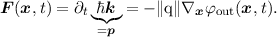
The force F(x,t) due to a gradient of the electrostatic potential or the band edges in the absence of
magnetic fields is given by
 | (2.26) |
where ∥q∥ is the sign-less elementary charge q, φ(x,t) the electrostatic potential and EC∕V the band
edge energy for either electrons or holes. Since the electrostatic potential is needed in order to
compute the force exerted on each charge carrier, one needs to solve Poisson’s equation
and the BTE for electrons and holes self-consistently. The full system of equations thus
reads,
∇⋅ = ∥q∥(n - p + C),
∂tfν
n + = ∥q∥(n - p + C),
∂tfν
n +  = = {fνn} = n{fν
n}- Γn{fν
n,fν
p },
∂tfν
p + {fνn} = n{fν
n}- Γn{fν
n,fν
p },
∂tfν
p +  ={fνp} = p{fν
n}- Γp{fν
n,fν
p }, ={fνp} = p{fν
n}- Γp{fν
n,fν
p }, | | (2.27) |
where additional scattering terms Γn∕p{fνn,fνp} have been added to account for recombination and
generation of electrons and holes. Since each BTE, without further approximations, has to be solved in
three spatial and three phase space dimensions in addition to the time dimension, a direct
discretization of the full system would lead to prohibitive memory and computational time
requirements for many applications. Thus further approximations or alternative discretization schemes
have to be employed to solve the system of equations.
2.2.1 Scattering
In this section a short introduction into modelling the scattering term {fν(x,k,t)} on the right
hand side of Equation (2.25) is given. While traveling through the lattice the electrons interact with
the lattice or other electrons. Such interactions, where the electrons change their momentum,
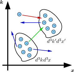
are termed scattering events. Considering an infinitesimal small volume d3kd3x in phase
space (cf. Figure 2.5), the electrons can either scatter into or out of this volume. Thus the
scattering operator is normally split into an in-scattering and out-scattering operator as
follows:
 |
The transitions in and out of an infinitesimal small volume d3kd3x in phase space do not occur
instantly. Nevertheless they are often modeled as an instant transition via a rate of expected
scattering charge carriers per second. Additionally it is assumed that the scattering occurs at
a certain point in real space and is a local event. For each flavor of scattering there is
a rate of transitions Sν(k,k′,t) from k to k′ in the phase space. An incomplete list of
interactions considered in this work can be found in Table 2.1. Note that in a homogeneous
semiconductor the scattering rate does not depend on the spatial location of the electron. This
simplifies the evaluation of the scattering terms. In order for an electron to scatter, the
initial state must be occupied by an electron and the final state must be empty by virtue of
Pauli’s exclusion principle. With all of the above the scattering operator is often modelled
as
{fν(x,k,t)} =  ∑
ν ∫ ∑
ν ∫
 |   in{fν(x,k,t)} in{fν(x,k,t)} | |
|
| - out{fν(x,k,t)}d3k′, out{fν(x,k,t)}d3k′, | (2.28) |
where the integral runs over the first Brillouin zone. In thermal equilibrium Equation (2.28) as
scattering operator in the BTE yields the Fermi-Dirac distribution
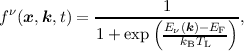 | (2.29) |
where EF is the Fermi-level and equals the chemical potential μ known from thermodynamics [12].
The computational burden to evaluate the integral in Equation (2.28) can strongly depend on
how the bandstructure is resolved and becomes easier to evaluate with the parabolic band
approximation. Nevertheless, upon solving the BTE the term fν(x,k′,t)(1 - fν(x,k,t)) in
Equation (2.28) might prove to be too challenging for a certain numerical BTE solver.
Thus the Pauli exclusion principle is often dropped and the scattering operator reduces
to
{fν(x,k,t)} =  ∑
ν ∫ ∑
ν ∫
| Sν(k′,k,t)fν(x,k′,t) | |
|
| - Sν(k,k′,t)fν(x,k,t)d3k′ | (2.30) |
and therefore gives the Maxwell-Boltzmann distribution as equilibrium distribution function
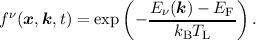 | (2.31) |
The integral in Equation (2.30) is easier to evaluate than Equation (2.28), especially when using the
parabolic band approximation and forms the basis of many important approximations, such as the
relaxation time approximation (RTA) [22]. Dropping Pauli’s exclusion principle is clearly justified if
(1 - fν(x,k,t)) ≈ 1 and thus fν(x,k,t)) ≪ 1 , which is only true for low electron (hole)
concentrations and non degenerate semiconductors. Thus dropping Pauli’s exclusion principle in
Equation (2.28) is often termed low density approximation.
| Interaction | Elastic/Inelastic | References |
|
|
|
| Acoustic Phonon Scattering | Approx. Elastic | [23, 24, 25] |
| Optical Phonon Scattering | Inelastic | [23, 24, 25] |
| Impurity Scattering | Approx. Elastic | [23, 26, 25] |
| Impact Ionization | Inelastic | [25, 27] |
| Electron-Electron Scattering | Inelastic | [28] |
| Table 2.1: | A list of particle interactions considered in this thesis including references to the
used models for the respective scattering rates. |
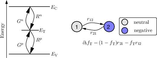
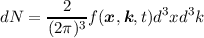
2.2.2 Recombination and Generation
The scattering operator as described in Section 2.2.1 does not consider electron-hole recombination
(cf. Equation (2.25)). In order to be able to consider recombination/generation processes the BTE
needs to be split into a BTE for electrons and holes respectively. Since recombination/generation
models can be quite complex [29], we first restrict this section to the most simple two-state defect
(cf. Figure 2.6), where only a single function over time, namely the trap occupancy fνT(t) and trap
level ET are needed to describe the state of the defect. Additionally it will be assumed that there are
enough electrons and holes that are either spin up or spin down, such that the trap occupancy is
independent of the electron spin. In case the spin cannot be neglected, the trap occupancy needs to be
split into its spin components, fνT(t) ⇒ fT,upν + fT,downν. With these assumptions the macroscopic
rate equation for the trap occupancy reads [12, 30]
| ∂tfν
T(t) | = ∑
ν ∫
(1 - fν
T(t))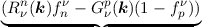 r21 r21 | (2.32)
|
| + fν
T(t)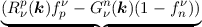 r12d3k, r12d3k, | | |
where Gνn(k) and Gνp(k) are the number of generated electrons and holes per second per d3k,
Rνn(k) and Rνp(k) are the number of recombined electrons and holes per second per d3k.
Putting all of the above together, the recombination operators Γp∕n{fνn,fνp} for electrons and holes,
which have been introduced in Equation (2.27), read
| Γn{fν
n,fν
p } | =  ∑
ν ∫
Gνn(k)fν
T(t)(1 - fν
n) - Rνn(k)(1 - fν
T(t))fν
nd3k, ∑
ν ∫
Gνn(k)fν
T(t)(1 - fν
n) - Rνn(k)(1 - fν
T(t))fν
nd3k, | (2.33)
|
| Γp{fν
n,fν
p } | =  ∑
ν ∫
Gνp(k)(1 - fν
T(t))(1 - fν
p ) - Rνp(k)fν
T(t)fν
p d3k, ∑
ν ∫
Gνp(k)(1 - fν
T(t))(1 - fν
p ) - Rνp(k)fν
T(t)fν
p d3k, | (2.34) |
where NT is the trap concentration. Dropping the sum over all bands in the equations above, the
recombination rates for electrons and holes are [31, 30]
 | (2.35) |
where σn and σp are experimentally determined capture cross sections and vn and vp reaction
velocities. From detailed balance [31, 12] the generation rates can be determined
 | (2.36) |