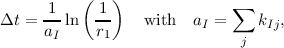
Each defect model, which can be derived based on first-order continuous-time Markov-Chains [143], can be stochastically interpreted. Thus two possibilities to solve the system of equations for the four-state NMP model as well as the SRH model [29] (cf. Chapter 2) are investigated here. The first possibility is to use a kinetic Monte Carlo algorithm to directly solve for the stochastic occupancies Xi(t) via the occupancy probabilities pi(t), whereas the second one is to solve for the occupancies fi(t) (cf. Section 6.2.4). One can choose, depending on the particular task, between those two methods independent of the choice for a particular transport model or BTE solving technique. Irrespective of the actual (non-linear) solver used for the transport model, the program flow stays essentially the same and is shown in Figure 6.12. In case the occupancies f(t) are of interest a straight forward assembly of the equations and the application of a linear solver suffice. For the kinetic Monte Carlo method, one first calculates the transition rates kIj between the currently occupied state I, ie. XI(t0) = 1, to all other possible states j. Then two uniformly distributed random numbers r1 and r2 between zero and one are drawn. Using random number r1 the time to the next state transition event,
|
| (6.50) |
is calculated such that XI(t0 + Δt) = 0 and XJ(t0 + Δt) = 1, where J is the final state. Afterwards, the final state J needs to be selected. For this one iterates, in arbitrary order, over all possible transitions j, where kIj∕aI are summed up until the random number r2 is smaller than the current sum. The final rate kIJ∕aI in the summation determines the final state J. The advantage of solving for the stochastic occupancies lies in the greater depth of information on the actual trapping event. By virtue of the algorithm trap self-interaction can be mitigated. This advantage however is then traded-off against the possibility to effectively use the simulator in a mixed-mode simulator and the possibility to carry out a small-signal analysis.
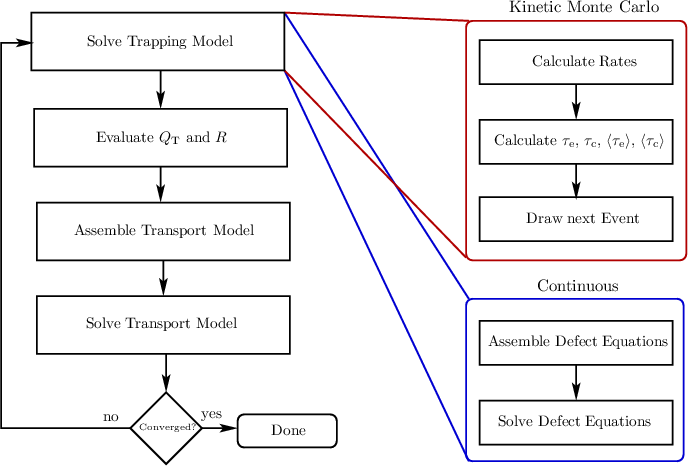
| Figure 6.12: | A flowchart for the implementation of NMP trapping models with suitable transport models. The transport model is, with the exception of the trapped charge and the recombination term, independent of the trapping model. This allows to use different techniques to solve the trapping model for the occupancies. When one solves for the stochastic occupancies a kinetic Monte Carlo algorithm can be used. |
The set of equations shown in the last sections are exponentially dependent on the electrostatic potential, which can be obtained by solving Poisson’s equations. Additionally, Poisson’s equation is tightly coupled to the transport model from which the quantities to calculate the NMP transition rates are obtained. The most pressing problem in the case of NMP transitions is the strong potential dependence of the NMP model, which results in self-interaction of the trap when solving for the occupancies fi(t). Since the occupancies fi(t) can take any value between zero and one, the trapped charge can also take all values between ±∥q∥ and zero. These fractional charges are added to the charge density in the Poisson equation and thus change the local electric field at the defect site, which in turn can cause a significant change in the transition rates and thus the capture and emission times. This tight coupling of quantities for self-consistency results in convergence problems of the non-linear solver, which is in the course of this thesis a Gummel-Iterator or a Newton-Raphson algorithm. However, solving for the time averaged occupancies does allow to effectively use the simulator in mixed-mode and the possibility to carry out a small-signal analysis, provided the full Jacobian is known. To demonstrate this, MinimosNT with a first-order quantum corrected drift diffusion model and the four-state NMP model (solving for fi(t)) have been used to simulate the time evolution of 2600 microscopically different defects [4]. The quantum correction has been accounted for by utilizing the density gradient model (cf. Chapter 4). To demonstrate the influence of potential fluctuations on the time constants predicted by the model, random discrete dopants have been considered too (cf. Figure 6.13). At last, Figure 6.14 shows the probabilities of self-interaction. However, as we have shown in [4] (cf. Figure 6.14) the error due to trap self-interaction is small and the validity of the simulation can be assessed. Nevertheless, if one is only interested in the evaluation of the capture and emission time of a single defect, self-consistency is often neglected and the trapping model can be evaluated after the transport model has been evaluated, without any coupling between trapping and transport model. Thus the system of equations for each defect described by an NMP based model is usually solved as a post processing step to the transport model whenever possible. Nevertheless, for example in the case of inhomogenous BTI this is not possible and one might need to utilize a KMC technique to solve the set of governing equations per trap.
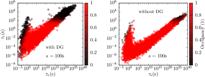
| Figure 6.13: | For each trap in one of 200 simulated microscopic devices with random discrete doping (left figure) and continuous doping (right figure), the occupancy after 100s of bias temperature stress is shown (color coded). It can be seen that traps with large emission time constants, which correspond to a more permanent degradation, are occupied. Here the capture time constants have been chosen to be within the stress time in order to demonstrate saturation. Additionally, it can be seen in the left figure that with random discrete doping the capture and emission time constants are more spread out, compared to continuous doping. |
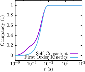
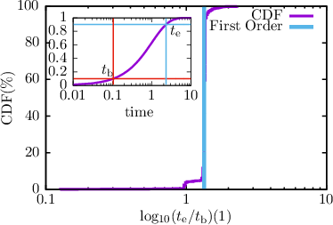
| Figure 6.14: | Left: The probability of a single self interacting trap to be occupied over stress time. The red curve is the occupancy for a self-consistent solution entering fractional charges leading to a trap self interaction during the charging process. As a reference the blue curve shows the expected charging behavior of the trap according to first-order kinetics. Right: The cumulative distribution function for the time it takes each trap to change its occupancy from 10% of its initial value to 90% of its final value on a log-scale (inset) for the whole ensemble of discrete traps in 200 simulations of a 35nm pMOSFET with an EOT of 1nm. Since significantly more than 90% of all 2600 traps exhibit the expected first-oder behavior, the influence of the self interacting traps is small. For simulation the drift diffusion simulator MinimosNT with density gradient for quantum correction and random discrete traps (four-state model) and dopants have been used. |
All bonds between atoms in an amorphous structure, such as the gate oxides used in MOSFETs, are of different configuration and exhibit, for example, great disparity in bond lengths. Thus the parameters of the trapping models used to describe BTI are not fixed but statistically distributed. Without any prior knowledge of the defect site configuration and its precursor configuration many parameters have to be estimated within physically reasonable bounds. An example for the four-state NMP model is given in Table 6.1. These parameters have also been used for the self-interaction example in the previous section. It is generally assumed that all parameters follow a Gaussian distribution, which is fully characterized by its respective mean value and standard deviation. For the simulation of an ensemble of traps, the same algorithm as for random discrete dopants is used to estimate the number of traps via a Poisson distribution, their spatial location via an uniform distribution and the parameter set for each defect via a Gaussian distribution. This approach, however, is not taken to describe TDDS data [105].
| Parameter | Mean Value μ | Standard Deviation σ |
| Et | 0.6 eV | 0.1 eV |
| Et′ | 0.75 eV | 0.1 eV |
| R | 0.5 | 0.01 |
| S | 0.6 | 0.01 |
| R′ | 0.8 | 0.01 |
| S′ | 0.6 | 0.01 |
| ϵT2 | 0.5 eV | 0.05 eV |
| ϵ1′1 | 0.8 eV | 0.05 eV |
| ϵ2′2 | 0.5 eV | 0.05 eV |
| Table 6.1: | Example mean values and standard deviations for the Gaussian distributed parameters of the four-state NMP model (Figure 6.11) used for demonstration purposes. The trap levels Et (that is d1) and Et′ (that is d1′) have the largest standard deviations, which results in a few traps being more likely in state 1′ than in state 1 before stress. Note that no correlations between the parameters have been assumed. |
Having a generalized algorithm for first-order time continuous Markov-Chain based BTI model (cf. Figure 6.12) the question remains: Which transport model is best suited to study BTI? Straightforwardly, any physical model which to sufficent accuracy describes the physical process underlying the unperturbed (no BTI) operation of a particular device is best suited to study BTI in that particular device. This is due to the nature of the NMP based models, which are, up to the inherent model error due to the assumptions made in the derivation, only as accurate as the physical device model, which delivers the necessary quantities, such as the electric field, the energy distribution function, charge carrier concentrations, lattice temperature and so on. Quantum corrected drift diffusion simulators, like MinimosNT, are well suited to study BTI in MOSFETs where the density gradient model is sufficent to describe carrier confinement, provided the drain voltage is low enough to guarantee low field transport [4]. However, for devices with pronounced quantum mehcanical effects, such as small diameter nanowires, SiGe MOSFETs [152] or nanoscale MOS structures, often Schrödinger-Poisson solvers are best suited if there is no transport, since they most accurately describe the device. Fortunately, Boltzmann Equation solvers, such as SHE, are only necessary in non-equilibrium if the charge carrier energy distribution functions for the device under BTI stress cannot be suitably approximated by a Maxwellian distributions anymore. In research this however is seldom the case, since BTI can be well studied, when there is little to no current flow in the device. Nevertheless, for device engineering the effect of BTI during usual use conditions, e.g. inhomogenous BTI, is of utmost importance to make lifetime predictions.