Subsections

• 3.5.1 Dirichlet Boundary Condition
• 3.5.2 Neumann Boundary Condition
• 3.5.3 Segregation Interface Condition
• 3.5.4 Surface Reactions

3.5 Boundary and Interface Conditions

In this section we present boundary conditions which are commonly used for the simulation of diffusion.

3.5.1 Dirichlet Boundary Condition

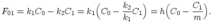
The physical meaning of the Dirichlet boundary condition is the diffusion from an infinite source of dopants. This might correspond to putting a heavily doped epitaxial layer on a lightly doped wafer.

3.5.2 Neumann Boundary Condition

The Neumann boundary condition for the considered dopant with concentration $C$,

$$\frac{\partial C}{\partial \mathbf{n}}= ,$$ (3.63)

means constant flux of the dopant in/out of the simulation domain. The most frequently used boundary condition in the diffusion simulation is zero the Neumann boundary condition, $\frac{\partial C}{\partial \mathbf{n}}=0$.

3.5.3 Segregation Interface Condition

Interfaces between different materials occur frequently in silicon processing. Dopants have different solubilities in different materials and so they redistribute at an interface until the chemical potential is the same on both sides of the interface. The ratio of the equilibrium doping concentration is defined as the segregation coefficient [31,32].
Next we consider two separate phases $S_0$ and $S_1$, which might be oxide and silicon. The transfer of the single species $X$ between $S_0$ and $S_1$ having concentrations $C_0$ in $S_0$ and $C_1$ in $S_1$ is decribed with a basic first order assumption is the species interchange at the interface according to the chemical reaction,

$$X_0\overset{k_1}{\underset{k_2}{\Longleftrightarrow}} X_1,$$ (3.64)

so the flux of material from $S_0$ to $S_1$ is,

$$F_{01}=k_1C_0-k_2C_1=k_1\Bigl(C_0-\frac{k_2}{k_1}C_1 \Bigr)=h\Bigl(C_0-\frac{C_1}{m} \Bigr).$$ (3.65)

In steady state $F_{01}=0$ and we obtain [31,32],

$$\frac{C_1}{C_0}=\frac{k_1}{k_2}.$$ (3.66)

where $h$ is the transfer coefficient over the interface, and $m$ is the segregation coefficient. Both of these coefficiens exibit temperature dependence according to Arrhenius law.

3.5.4 Surface Reactions

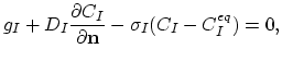
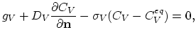
The chemical reaction at the surface of the simulation domain, when a net flux $g_I$ or $g_V$ of either interstitial or vacancies, respectively is injected, is decribed by the equations,

$$g_{I} + D_{I} \frac{\partial C_I}{\partial \mathbf{n}} - \sigma_{I}(C_{I}-C_{I}^{eq}) = 0,$$ (3.67)

$$g_{V} +D_{V} \frac{\partial C_V}{\partial \mathbf{n}} - \sigma_{V}(C_{V}-C_{V}^{eq}) = 0,$$ (3.68)

where surface loss terms are modeled with surface recombination velocities $\sigma_{I}$ and $\sigma_{V}$. The equations (3.67) and (3.68) are used in standard OED and ORD models [20].

Surface processes are dominant in determining the concentration of point defects in typical silicon wafers [33]. Evidence that pad-oxides/silicon interfaces are good sinks for interstitials comes from observations on the growth and shrinkage of stacking faults in silicon under different surface coverings[34].