Subsections

• 3.4.1 Simple Point Defect Model
• 3.4.2 Three-Stream Mulvaney-Richardson Model
• 3.4.3 Five-Stream Dunham Model

3.4 Nonequilibrium Models

After implantation substitional dopant atoms are immobile. The dopant diffusion process is only possible when substitional dopant atoms interact with native point defects by building dopant-point defect pairs. Silicon point defects are temporarily consumed to generate mobile species (dopant-point defect pairs), which then migrate into the silicon wafer interior, where the mobile dopants settle down on lattice sites to become a substitutional dopants, releasing silicon point defects in the process [25,24,26,20].

In the cases where a strong source of point defects exists on the wafer surface, transport of the dopant-point defects pairs causes a supersaturation of the point defects in the bulk region, and subsequentially kinks and ledges of the dopant profiles become apperant. The tails of dopant profiles diffuse much faster than expected, which is exactelly what is observed experimentally [29,26,27,30].

Due to the active participation in the dopant diffusion, native silicon point defects exhibit dynamics which significantelly depart from the equilibrium state [21,6]. In the following sections three widely applied non-equilibrium models for the point defect assisted dopant diffusion are presented.

3.4.1 Simple Point Defect Model

The simplest way to model the impact of the non-equilibrium interstitials' and vacancies' dynamic is using the cumulative diffusion coefficient,

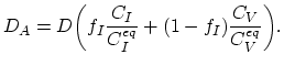$$D_A=D\biggl(f_I \frac{C_I}{C_{I}^{eq}} + (1 - f_I)\frac{C_V}{C_{V}^{eq}} \biggr).$$ (3.39)

Here, $C_{I}^{eq}$ and $C_{V}^{eq}$ are equilibrium values of interstitial and vacancy concentrations, respectively. The parameter $f_I$ takes the value of one, if the diffusion works exclusively via interstitials, and zero if it works exclusively via vacancies.

The model assumes that the dopant-defect pairing reactions and pair dissociation/defect recombination are in local equilibrium. The recombination and generation of Frankel pairs are modeled by,

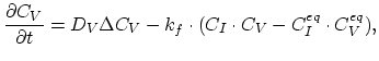$$\frac{\partial C_V}{\partial t}=D_V \Delta C_V - k_{f} \cdot ( C_I \cdot C_V - C_{I}^{eq} \cdot C_{V}^{eq}),$$ (3.40)

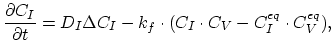$$\frac{\partial C_I}{\partial t}=D_I \Delta C_I - k_{f} \cdot ( C_I \cdot C_V - C_{I}^{eq} \cdot C_{V}^{eq}),$$ (3.41)

denoting the reaction constant as $k_f$, and the diffusion coefficient of interstitials and vacancies as $D_I$ and $D_V$, respectively. Taking the diffusion coefficient $D_A$ as defined by (3.39) the dopant diffusion is modeled by a simple diffusion equation,

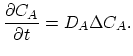$$\frac{\partial C_A}{\partial t}= D_A \Delta C_A.$$ (3.42)

This model is correct in the case of enhanced and oxidation retarded diffusion for low concentrations of dopants [20].

3.4.2 Three-Stream Mulvaney-Richardson Model

Under most annealing conditions, with exception of the rapid thermal annealing ($RTA$), the dopant-defect pairing reactions are fast enough to maintain the pair concentration near local equilibrium with the concentrations of isolated dopands and defects,

$$C_{(AI)^{i+1}}=K_{A+I}^i C_{A^{+}}C_{I^{i}},$$ (3.43)

$$C_{(AV)^{i+1}}=K_{A+V}^i C_{A^{+}}C_{V^{i}}.$$ (3.44)

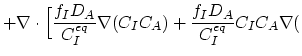
Further simplifications is to aggregate different charge states of the species taking part in reactions to one single concentration. The last step was done in [29] in order to obtain model described by following equations,

$$\frac{\partial C_A}{\partial t}= \nabla\cdot \Bigl[ \frac{f_I D_A}{C_{I}^{eq}}\nabla (C_I C_A) + \frac{f_I D_A}{C_{I}^{eq}}C_I C_A \nabla ( n)\Bigr] +$$

$$+\nabla\cdot \Bigl [\frac{(1-f_I)D_A}{C_{V}^{eq}} \nabla (C_V C_A) + \frac{(1-f_I)D_A}{C_{V}^{eq}} C_V C_A\nabla ( n)\Bigr],$$ (3.45)

$$\frac{\partial C_I}{\partial t}=\nabla\cdot(D_I\nabla C_I) - k_{f} ( C_I C_V - C_{I}^{eq} C_{V}^{eq}) +$$

$$+\nabla\cdot \Bigl [ \frac{f_I D_A}{C_{I}^{eq}}\nabla (C_I C_A) + \frac{f_I D_A}{C_{I}^{eq}}C_I C_A \nabla ( n)\Bigr],$$ (3.46)

$$\frac{\partial C_V}{\partial t}=\nabla\cdot(D_V\nabla C_V) - k_{f} ( C_I C_V - C_{I}^{eq} C_{V}^{eq}) +$$

$$+\nabla\cdot \Bigl [\frac{(1-f_I)D_A}{C_{V}^{eq}} \nabla (C_V C_A) + \frac{(1-f_I)D_B}{C_{V}^{eq}} C_V C_A\nabla ( n)\Bigr].$$ (3.47)

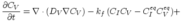
$f_I$ is the fractional contribution of the interstitial mechanism to the dopants diffusion. The approach of Mulvaney and Richardson [29] successfully models kink and tail diffusion of boron and phosphorus (Figure 3.1).

Figure 3.1: Diffusion of phosphorus at $900^{\circ }$ C for one hour. Phosphorus diffuses primarily through pairing with intrinsic interstitials. The nonequlibrium dynamics of the intrinsic interstitials accounts for characteristic kink and tail parts of the final profile.

3.4.3 Five-Stream Dunham Model

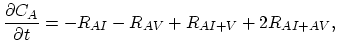
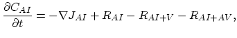
Taking into account non-equilibrium reactions of dopants and point defects we have to deal with a system of five equations (five-stream model). These are continuity equations for the total concentrations of A$^{+}$, AI, AV, I, V, over all charge states for each species [30],

$$\frac{\partial C_A}{\partial t} = -R_{AI}-R_{AV}+R_{AI+V}+2R_{AI+AV},$$ (3.48)

$$\frac{\partial C_{AI}}{\partial t} = -\nabla J_{AI}+R_{AI}-R_{AI+V}-R_{AI+AV},$$ (3.49)

$$\frac{\partial C_{AV}}{\partial t} = -\nabla J_{AV}+R_{AV}-R_{AV+I}-R_{AI+AV},$$ (3.50)

$$\frac{\partial C_I}{\partial t} = -\nabla J_{I} - R_{AI}-R_{I+V},$$ (3.51)

$$\frac{\partial C_V}{\partial t} = -\nabla J_{V} - R_{AV}-R_{I+V}.$$ (3.52)

$R_{AI}$ and $R_{AV}$ dopant/point defect pairing reactions rates defined as,

$$R_{AI} = \Bigl[ \sum_i k_{AI}^i K_{I}^i\Bigl(\frac{n_i}{n} \Bigr)^i \Bigr] \Bigl[ C_{A^+}C_{I^0}-\frac{C_{(AI)^+}}{K_{A+I}^0}\Bigr],$$ (3.53)

$$R_{AV} = \Bigl[ \sum_i k_{AV}^i K_{V}^i\Bigl(\frac{n_i}{n} \Bigr)^i \Bigr] \Bigl[ C_{A^+}C_{V^0}-\frac{C_{(AV)^+}}{K_{A+V}^0}\Bigr].$$ (3.54)

$R_{I+V}$ is Frankel recombination rate defined as,

$$R_{I+V}= \Bigl[ \sum_{i,j} k_{I+V}^{i,j} K_{I}^i K_{V}^j\Bigl(\frac{n_i}{n} \Bigr)^{i+j} \Bigr][C_{I^0}C_{V^0}-C_{I^0}^{eq}C_{V^0}^{eq}].$$ (3.55)

Finally, $R_{AI+V}$, $R_{AV+I}$, and $R_{AI+AV}$ are net rates of the pair/defect and pair/pair reactions.

$$R_{AI+V}=\Bigl[ \sum_{i,j} k_{AI+V}^{i,j} K_{AI}^i K_{V}^j\Bigl(\... ...igr)^{i+j} \Bigr][C_{(AI)^+}C_{V^0}-K_{A+I}^0 C_{I^0}^{eq}C_{V^0}^{eq}C_{A^+}],$$ (3.56)

$$R_{AV+I}=\Bigl[ \sum_{i,j} k_{AV+I}^{i,j} K_{AV}^i K_{I}^j\Bigl(\... ...igr)^{i+j} \Bigr][C_{(AV)^+}C_{I^0}-K_{A+V}^0 C_{V^0}^{eq}C_{I^0}^{eq}C_{A^+}],$$ (3.57)

$$R_{AI+AV}=\Bigl[ \sum_{i,j} k_{AI+AV}^{i,j} K_{AI}^i K_{AV}^j\Bigl(\frac{n_i}{n}\Bigr)^{i+j} \Bigr] [C_{(AI)^{+}}C_{(AV)^{+}}-$$

$$K_{A+I}^{0} K_{A+V}^{0} C_{I^0}^{eq} C_{V^0}^{eq} (C_{A^+})^2].$$ (3.58)

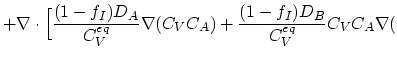
We also need terms for the fluxes $J_{AI}$, $J_{AV}$, $J_{I}$, and $J_{V}$. Flux $J_{P}$ does not appear in the equations, because it is assumed that isolated dopant atoms are immobile and therefore $J_{P}=0$ holds everywhere in the silicon bulk,

$$J_{AI}=-\Bigl[ \sum_{i} D_{(AI)^{i+1}} K_{AI}^i \Bigl(\frac{n_i}{... ...+C_{(AI)^{+}}\Bigl(\frac{n_i}{n} \Bigr)\nabla \Bigl(\frac{n}{n_i} \Bigr)\Bigr],$$ (3.59)

$$J_{AV}=-\Bigl[ \sum_{i} D_{(AV)^{i+1}} K_{AV}^i \Bigl(\frac{n_i}{... ...+C_{(AV)^{+}}\Bigl(\frac{n_i}{n} \Bigr)\nabla \Bigl(\frac{n}{n_i} \Bigr)\Bigr],$$ (3.60)

$$J_{I}=-\Bigl[ \sum_{i} D_{I^{i}} K_{I}^i \Bigl(\frac{n_i}{n} \Bigr) \Bigr] \nabla C_{I^{0}},$$ (3.61)

$$J_{V}=-\Bigl[ \sum_{i} D_{V^{i}} K_{V}^i \Bigl(\frac{n_i}{n} \Bigr) \Bigr] \nabla C_{V^{0}}.$$ (3.62)

In the equations (3.54)-(3.60) $k_X$ represents forward reaction rate coefficients, and $K_X$ represents equilibrium constants.
The model considered in this section correctly predicts the rapid diffusion in the peak region observed at high concentrations of phosphorus as well as the dependence of tail diffusion on the peak doping level, while remaining consistent with experimental results indicating that phosphorus diffusion is dominated by interstitials [30].